Honey, I shrunk the target variable

Motivation

For me, it is often an irritating sight to see how inexperienced, up and coming data scientists jump right into the feature engineering when facing some new supervised learning problem… but it also makes me contemplate about my past when I started doing data science. So full of vigour and enthusiasm, I was often completely absorbed by the idea of minimizing whatever error measure I was given or maybe some random one I chose myself, like the root mean square error. In my drive, I used to construct many derived features using clever transformations and sometimes did not even stop at the target variable. Why should I? If the target variable is for instance non-negative and quite right-skewed, why not transform it using the logarithm to make it more normally distributed? Isn’t this better or even required for simple models like linear regression, anyways? A little $\log$ never killed a dog, so what could possibly go wrong?

As you might have guessed from these questions, it’s not that easy, and transforming your target variable puts you directly into the danger zone. In this blog post, I want to elaborate on why this is so from a mathematical perspective but also by demonstrating it in some practical examples. Without spoiling too much I hope, for the too busy or plain lazy readers, the main take-away is:

TLDR: Applying any non-affine transformation to your target variable might have unwanted effects on the error measure you are minimizing. So if you don’t know exactly what you are doing, just don’t.

Let’s get started

Before we start with the gory mathematical details, let’s first pick and explore a typical use-case where most inexperienced data scientists might be tempted to transform the target variable without a second thought. In order to demonstrate this, I chose the used-cars database from Kaggle and if you want to follow along, you find the code in the notebooks folder of my Github used-cars-log-trans repository. As the name suggests, the data set contains used cars having car features like vehicleType, yearOfRegistration & monthOfRegistration, gearbox, powerPS, model, kilometer (mileage), fuelType, brand and price.

Let’s say the business unit basically asks us to determine the proper market value of a car given the features above to determine if its price is actually a good deal, fair deal or a bad deal. The obvious way to approach this problem is to create a model that predicts the price of a car, which we assume to be its market value, given its features. Since we have roughly 370,000 cars in our data set, for most cars we will have many similar cars and thus our model will predict a price that is some kind of average of their prices. Consequently, we can think of this predicted price (let’s call it pred_price) as the actual market value. To determine if the actual price of a vehicle is a good, fair or bad deal, we would then calculate for instance the relative error

$$\frac{\mathrm{pred\_price} - \mathrm{price}}{\mathrm{price}}$$

in the simplest case. If the relative error is close to zero we would call it fair, if it is much larger than zero it’s a good deal and a bad deal if it is much smaller than zero. For the actual subject of this blog post, this use-case serves us already as a good motivation for the development of some regression model that will predict the price given some car features. The attentive reader has certainly noticed that the prices in our data set will be biased towards a higher price and thus also our predicted “market value”. This is due to the fact that we don’t know for which price the car was eventually sold. We only know the amount of money the seller wanted to have which is of course higher or equal than what he or she gets in the end. For the sake of simplicity, we assume that we have raised this point with the business unit, they noted it duly and we thus neglect it for our analysis.

Choosing the right error measure

At this point, a lot of inexperienced data scientists would directly get into business of feature engineering and build some kind of fancy model. Nowadays most machine learning frameworks like Scikit-Learn are so easy to use that one might even forget the error measure that is optimized as in most cases it will be the mean square error (MSE) by default. But does the MSE really make sense for this use-case? First of all is our target measured in some currency, so why would we try to minimize some squared difference? Squared Euro? Very clearly, even taking the square root in the end, i.e. root mean square error (RMSE), would not change a thing about this fact. Still, we would weight one large residual higher than many small residuals which sum up to the exact same value as if 10 times a residual of 10.- € is somehow less severe than a single residual of 100.- €. You see where I am getting at. In our use-case an error measure like the mean absolute error (MAE) might be the more natural choice compared to the MSE.

On the other hand, is it really that important if a car costs you 1,000.- € more or less? It definitely does if you are looking at cars at around 10,000.- € but it might be negligible if your luxury vehicle is around 100,000.- € anyway. Consequently, the mean absolute percentage error (MAPE) might even be a better fit than the MAE for this use-case. Having said that, we will keep all those error measures in mind but use the default MSE criterion in our machine-learning algorithm for the sake of simplicity and to help me make the actual point of this blog post ;-)

Nevertheless, one crucial aspect should be kept in mind for the rest of this post. In the end after the fun part of modeling, we, as data scientists, have to communicate the results to business people and the assessment of the quality of the results is going to play an important role in this. This assessment will almost always be conducted using the raw, i.e. untransformed, target as well as the chosen error measure to answer the question if the results are good enough for the use-case at hand and consequently if the model can go to production as a first iteration. Practically, that means that even if we decide to train a model on a transformed target, we have to transform the predictions of the model back for evaluation. Results are always communicated based on the original target.

Distribution of the target variable

Our data contains not only cars that are for sale but also cars people are searching for with a certain price. Additionally, we have people offering damaged cars, wanting to trade their car for another or just hoping to get an insanely enormous amount of money. Sometimes you get lucky. For our use-case, we gonna keep only real offerings of undamaged cars with a reasonable price between 200.- € and 50,000.- € with a first registration not earlier than 1910. This is what the distribution of the price looks like.

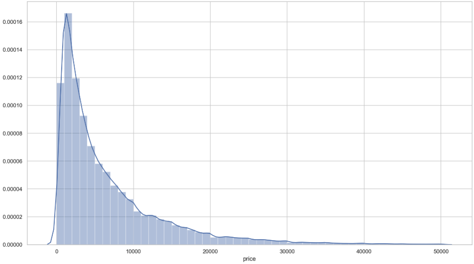
distribution of price — Distribution plot of the price variable using 1,000.- € bins.

It surely does look like a log-normal distribution and just to have visual check, fitting a log-normal distribution with the help of the wonderful SciPy gets us this.

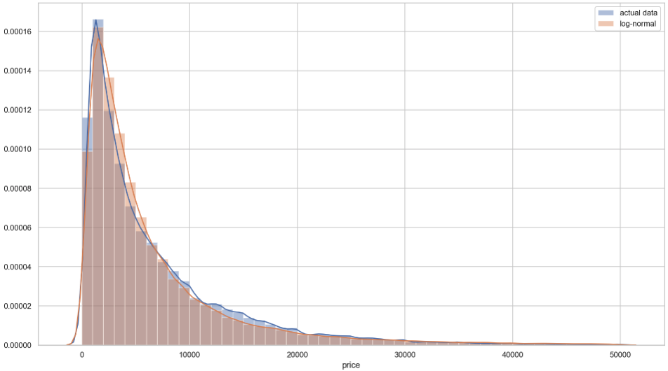
log-normal fit — Log-normal distribution fitted to the distribution of prices.

Seeing this, you might feel the itch to just apply now the logarithm to our target variable, just to make it look more normal. And isn’t this some basic assumption of a linear model anyway?

Well, this is a common misconception. The dependent variable, i.e. target variable, of a linear model doesn’t need to be normally distributed, only the residuals are. This can be seen easily by revisiting the formula of a linear model. For the observed outcome $y_i$ and some true latent outcome $\mu_i$ of the $i$-th sample, we have

\begin{equation} \begin{split} \mu_i &= \sum_{j=1}^M w_j \phi_j(\mathbf{x}_i) , \\ y_i &= \mu_i + \epsilon, \end{split}\label{eqn:linear-model} \end{equation}

where $\mathbf{x}_i$ is the original feature vector, $\phi_j$, $j=1, \ldots, M$ a set of (potentially non-linear) functions, $w_j$, $j=1, \ldots, M$ some scalar weights and $\epsilon$ some random noise that is distributed like the normal distribution with mean $0$ and variance $\sigma^2$ (or $\epsilon\sim\mathcal{N}(0, \sigma^2)$ for short). If you wonder about the $\phi_j$, that’s where all your feature engineering skills and domain knowledge go into to transform the raw features into more suitable ones.

One of the reasons for this common misconception might be that the literature often states that the dependent variable $y$ conditioned on the predictor $\mathbf{x}$ is normally distributed in a linear model. So for a fixed $\mathbf{x}$ we have according to $\eqref{eqn:linear-model}$ also a fixed $\mu$ and thus $y$ can be imagined as a realization of a random variable $Y=\mathcal{N}(\mu, \sigma^2)$.

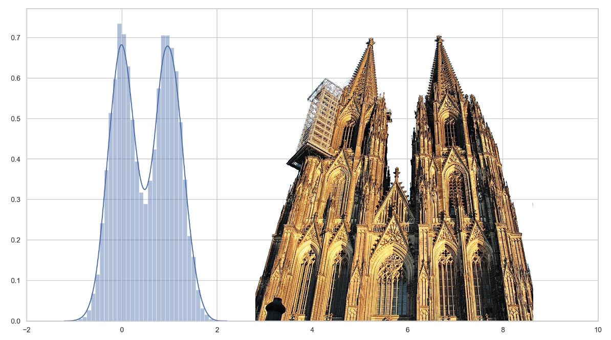
To make it even a tad more illustrative, imagine you want to predict the average alcohol level (in some strange log scale) of a person celebrating Carnival only using a single binary feature, e.g. did the person have a one-night-stand over Carnival or not. Under these assumptions we simple generate some data using the linear model from above and plot it:

import numpy as np
import seaborn as sns
import matplotlib.pylab as plt

N = 10000  # number of people
x = np.random.randint(2, size=N)
y = x + 0.28*np.random.randn(N)

sns.distplot(y)
plt.xlim(-2, 10)

Obviously, this results in a bimodal distribution also known as the notorious Cologne Cathedral distribution as some may call it. Thus, although using a linear model, we generated a non-normally distributed target variable with residuals that are normally distributed.

Based on common mnemonic techniques, and assuming this example was surprising, physical, sexual and humorous enough for you, you will never forget that the residuals of a linear model are normally distributed and not the target variable in general. Only in the case that you used a linear model having only an intercept, i.e. $M=1$ and $\phi_1(\mathbf{x})\equiv 1$, the target distribution equals the residual distribution (up to some shift) on all data sets. But seriously, who does that in real life?

Analysis of the residual distribution

Now that we learnt about the distribution of the residual, we want to further analyse it. Especially with respect to the error measure that we are trying to minimize as well as the transformation we apply to the target variable beforehand. Let’s take a look at the definition of the MSE again, i.e.

\begin{equation} \frac{1}{n}\sum_{i=1}^n (y_i - \hat y_i)^2,\label{eqn:sum_residual} \end{equation}

where $\hat y_i = \hat y(\mathbf{x}_i)$ is our prediction given the feature vector $\mathbf{x}_i$ and $y_i$ is the observed outcome for the sample $i$. In reality we might only have a single or maybe a few samples sharing exactly the same feature vector $\mathbf{x}_i$ and thus also the same model prediction $\hat y_i$. In order to do some actual analysis, we now assume that we have an infinite number of observed outcomes for a given feature vector. Now assume we keep $\mathbf{x}_i$ fixed and want to compute $\eqref{eqn:sum_residual}$ having all those observed outcomes. Let’s drop the index $i$ from $\hat y_i$ as it depends only on our fixed $\mathbf{x}_i$. Also we can imagine all these outcomes $y$ to be realizations of some random variable $Y$ conditioned on $\mathbf{x}$. To now handle an infinite number of possible realizations, we need to introduce the probability $f(y)$ of some realization $y$, or more precisely the probability density function (pdf) since $Y$ is a continuous random variable. Consequently, as the summation becomes an integration, the discrete MSE in $\eqref{eqn:sum_residual}$ becomes

\begin{equation} \int_{-\infty}^\infty (y - \hat y)^2f(y)\, \mathrm{d}y,\label{eqn:int_residual} \end{equation}

as you might have expected. Now this is awesome, as it allows us to apply some good, old-school calculus. By the way, when I am talking about the residual distribution I am actually referring to the distribution $y - \hat y$ with $y\sim f(y)$. Thus the residual distribution is determined by $f(y)$ except for a shift of $\hat y$. So what kind of assumptions can we make about it? In case of a linear model as in $\eqref{eqn:linear-model}$, we assume $f(y)$ to be the pdf of a normal distribution but it could also be anything else. In our car pricing use-case, we know that $y$ will be non-negative as no one is gonna give you money if you take a working car. Let me know if you have a counter-example ;-) This rules out the normal distribution and demands a right skewed distribution, thus the pdf of the log-normal distribution might be an obvious assumption for $f(y)$ but we will come back later to that.

For now, we gonna consider $\eqref{eqn:int_residual}$ again and note that our model, whatever it is, will somehow try to minimize $\eqref{eqn:int_residual}$ by choosing a proper $\hat y$. So let’s do that analytically by deriving $\eqref{eqn:int_residual}$ with respect to $\hat y$ and setting to $0$, we have that

$$ \frac{d}{d\hat y}\int_{-\infty}^\infty (y - \hat y)^2f(y)\, \mathrm{d}y = -2\int_{-\infty}^\infty yf(y)\, \mathrm{d}y + 2\hat y \stackrel{!}{=} 0, $$

and subsequently

\begin{equation} \hat y = \int_{-\infty}^\infty yf(y)\, \mathrm{d}y.\label{eqn:expected-value} \end{equation}

Looks familiar? Yes, this is just the definition of the expected value in the continuous case! So whenever we are using the RMSE or MSE as error measure, we are actually calculating the expected value of $y$ at some fixed $\mathbf{x}$. So what happens if we do the same for the MAE? In this case, we have

$$ \int_{-\infty}^\infty \vert y-\hat y\vert f(y)\, \mathrm{d}y=\int_{\hat y}^\infty (y-\hat y) f(y)\, \mathrm{d}y-\int_{-\infty}^{\hat y} (y-\hat y)f(y)\, \mathrm{d}y, $$

and deriving by $\hat y$ again, we have

$$ \int_{-\infty}^{\hat y} f(y)\, \mathrm{d}y - \int_{\hat y}^\infty f(y)\, \mathrm{d}y \stackrel{!}{=} 0. $$

We thus have $\hat y = P(X\leq \frac{1}{2})$, which is, lo and behold, the median of the distribution with pdf $f(y)$!

A small recap at this point. We just learnt that minimizing the MSE or RMSE (also l2-norm as a fancier name) leads to the estimation of the expected value while minimizing MAE (also known as l1-norm) gets us the median of some distribution. Also remember that our feature vector $\mathbf{x}$ is still fixed, so $y\sim f(y)$ just describes the random fluctuations around some true value $y^\star$, which we just don’t know, and $\hat y$ is our best guess for it. If we assume the normal distribution there is no reason to abandon all the nice mathematical properties of the l2-norm since the result will be theoretically the same as minimizing the l1-norm. It may make a huge difference though, if we are dealing with a non-symmetrical distribution like the log-normal distribution.

Let’s just demonstrate this using our used cars example. We have already seen that the distribution of price is rather log-normally than normally distributed. If we now use the simplest model we can think of, having only a single variable, (yeah, here comes the linear model with just an intercept again), the target distribution directly determines the residual distribution. Now, we find the minimum point using RMSE and MAE to compare the results to the mean and median of the price vector y, respectively.

>>> def rmse(y_pred, y_true):
>>>     # not taking the root, i.e. MSE, would not change the actual result
>>>     return np.sqrt(np.mean((y_true - y_pred)**2))

>>> def mae(y_pred, y_true):
>>>     return np.mean(np.abs(y_true - y_pred))

>>> y = df.price.to_numpy()
>>> sp.optimize.minimize(rmse, 1., args=(y,))
      fun: 7174.003600843465
 hess_inv: array([[7052.74958795]])
      jac: array([0.])
  message: 'Optimization terminated successfully.'
     nfev: 36
      nit: 5
     njev: 12
   status: 0
  success: True
        x: array([6703.59325181])

>>> np.mean(y)
6704.024314214464

>>> sp.optimize.minimize(mae, 1., options=dict(gtol=2e-4), args=(y,))
      fun: 4743.492333474732
 hess_inv: array([[7862.69627309]])
      jac: array([-0.00018311])
  message: 'Optimization terminated successfully.'
     nfev: 120
      nit: 8
     njev: 40
   status: 0
  success: True
        x: array([4099.9946168])

>>> np.median(y)
4100.0

As expected, by looking at the x in the output of minimize, we approximated the mean by minimizing the RMSE and the median by minimizing the MAE.

Shrinking the target variable

There is still some elephant in the room that we haven’t talked about yet. What happens now if we shrink our target variable by applying a log transformation and then minimize the MSE?

>>> y_log = np.log(df.price.to_numpy())
>>> sp.optimize.minimize(rmse, 1., args=(y_log,), tol=1e-16)
      fun: 1.0632889349620418
 hess_inv: array([[1.06895454]])
      jac: array([0.])
  message: 'Optimization terminated successfully.'
     nfev: 36
      nit: 6
     njev: 12
   status: 0
  success: True
        x: array([8.31228458])

So if we now transform the result x which is roughly 8.31 back using np.exp(8.31) we get a rounded result of 4064. Wait a second! What just happened!? We would have expected the final result to be around 6704 because that’s the mean value we had before. Somehow, transforming the target variable, minimizing the same error measure as before and applying the inverse transformation changed the result. Now our result of 4064 looks rather like an approximation of the median… well… it actually is assuming a log-normal distribution as we will fully understand soon. If we had applied some full-blown machine learning model, the difference would have been much smaller since the variance of the residual distribution would have been much smaller. Still, we would have missed our actual goal of minimizing the (R)MSE on the raw target. Instead we would have unknowingly minimized the MAE, which might actually be better suited for our use-case at hand. Nevertheless, being a data scientist, we should know what we are doing and a lucky punch without a clue of what happened, just doesn’t suit a scientist.

Before, we showed that the distribution of prices, and thus our target, resembles a log-normal distribution. So let’s assume now that we have a log-normal distribution, and thus we have $\log(\mathrm{price})\sim\mathcal{N}(\mu,\sigma^2)$. Consequently, the pdf of the price is

\begin{equation} \tilde f(x) = \frac {1}{x}\cdot {\frac {1}{ {\sqrt {2\pi\sigma^2 \,}}}}\exp \left(-{\frac {(\ln(x) -\mu )^{2}}{2\sigma ^{2}}}\right),\label{eqn:log-normal} \end{equation}

where the only difference to the pdf of the normal distribution is $ln(x)$ instead of $x$ and the additional factor $\frac{1}{x}$. Also note that parameters $\mu$ and $\sigma$ are the well-known parameters of the normal distribution but for the log-transformed target. So when we now minimize the RMSE of the log-transformed prices as we did before, we actually infer the parameter $\mu$ of the normal distribution, which is the expected value and also the median, i.e. $\operatorname {P} (\log(\mathrm{price})\leq \mu)= 0.5$. Applying any kind of strictly monotonic increasing transformation $\varphi$ to the price, we see that $\operatorname {P} (\varphi(\log(\mathrm{price}))\leq \varphi(\mu)) = 0.5$ and thus the median as well as any other quantile is equivariant under the transformation $\varphi$. In our specific case from above, we have $\varphi(x) = \exp(x)$ and thus the result, that we are approximating the median instead of the mean, is not surprising at all from a mathematical point of view.

The expected value is not so well-behaved under transformations as the median. Using the definition of the expected value $\eqref{eqn:expected-value}$, we can easily show that only transformations $\phi$ of the form $\phi(x)=ax + b$, with scalars $a$ and $b$, allow us to transform the target, determine the expected value and apply the inverse transformation to get the expected value of the original distribution. In math-speak, a transformation of the form $\phi(x)=ax + b$ is also called an affine transformation. For the transformed random variable $\phi(X)$ we have for the expected value that

$$ \begin{align*} E[\phi(X)] &= E[aX + b] \\ &= \int (ax + b)f(x)\, \mathrm{d}x \\ &= a\int xf(x)\, \mathrm{d}x + b \\ &=aE[X] + b =\phi(E[X]), \end{align*} $$

where we used the fact that probability density functions are normalized, i.e. $\int f(x)\mathrm{d}x=1$. What a relief! That means at least affine transformations are fine when we minimize the (R)MSE. This is especially important if you belong to the illustrious circle of deep learning specialists. In some cases, the target variable of a regression problem is standardized or min-max scaled during training and transformed back afterwards. Since these normalization techniques are affine transformations we are on the safe side, though.

Let’s come back to our example where we know that the distribution is quite log-normal. Can we somehow still receive the mean of the untransformed target variable? Yes we can, actually. Using the parameter $\mu$ that we already determined above we just calculate the variance $\sigma^2$ and have $\exp(\mu + \frac{\sigma^2}{2})$ for the mean of the untransformed distribution. More details on how to do this can be found in the notebook of the used-cars-log-trans repository. Way more interesting, at least for the mathematically interested reader, is the question Why does this work?.

This is easy to see using some calculus. With $\tilde y = \log(y)$ and let $f(y)$ be the pdf of the normal distribution as well as $\tilde f(y)$ the pdf of the log-normal distribution $\eqref{eqn:log-normal}$. Using integration by substitution and noting that $\mathrm{d}y = e^{\tilde y}\mathrm{d}\tilde y$, we have

\begin{equation} \int y \tilde f(y)\, \mathrm{d}y = \int e^{\tilde y} \tilde f(e^{\tilde y})e^{\tilde y}\, \mathrm{d}\tilde y = \int e^{\tilde y} f(\tilde y)\, \mathrm{d}\tilde y,\label{eqn:mean-log-normal} \end{equation}

where in the last equation the additional factor of the log-normal distribution was canceled out with $e^{\tilde y}$ and thus became the pdf of the normal distribution due to our substitution. Writing out the exponent in $f(x)$, which is $-\frac{(\tilde y-\mu)^2}{2\sigma^2}$ and completing the square with $\tilde y$, we have

\begin{equation} \begin{split} \tilde y - \frac{(\tilde y-\mu)^2}{2\sigma^2} &= -\frac{\mu^2 - 2\mu\tilde y + \tilde{y}^2 - 2\sigma^2\tilde y}{2\sigma^2} \\ &= -\frac{(\tilde y - (\mu + \sigma^2))^2}{2\sigma^2} + \mu + \frac{\sigma^2}{2}. \end{split}\label{eqn:completing_square} \end{equation}

Using this result, we can rewrite the last expression of $\eqref{eqn:mean-log-normal}$ by shifting the parameter $\mu$ of the normal distribution by $\sigma^2$. Denoting with $f_s(y)$ the shifted pdf, we have

$$ \int e^{\tilde y} f(\tilde y)\, \mathrm{d}\tilde y = e^{\mu + \frac{1}{2}\sigma^2}\int f_s(\tilde y)\, \mathrm{d}\tilde y = e^{\mu + \frac{\sigma^2}{2}}, $$

and subsequently we have proved that the expected value of the log-normal distribution indeed is $\exp(\mu + \frac{\sigma^2}{2})$.

A little recap of this section’s most important points to remember. When minimizing l2, i.e. (R)MSE, only affine transformations allow us the determine the expected value of the original target by applying the inverse transformation to the expected value of the transformed target variable. When minimizing l1, i.e. MAE, all strictly monotonic increasing transformations can be applied to determine the median from the transformed target variable followed by the inverse transformation.

Transforming the target for fun and profit

So we have seen that not everything is as it seems or as we might have expected by doing some rather academical analysis. But can we somehow use this knowledge in our use-case of predicting the market value of a used car? Yeah, this is the point where we close the circle to the beginning of the story. We already argued that the RMSE might not be the right error measure to minimize. Log-transforming the target and still minimizing the RMSE gave us an approximation to the result we would have gotten if we had minimized the MAE, which quite likely is a more appropriate error measure in this use-case than the RMSE. This is a neat trick if our regression method only allows minimizing the MSE or if it is too slow or unstable when minimizing the MAE directly. A word of caution again, this only works if the residual distribution approximates a log-normal distribution. So far we have only seen that the target distribution, not the residual distribution, is quite log-normal but since we are dealing with positive numbers, and also taking into account the fact that a car seller might be more inclined to start with a higher price, this justifies the assumption that the residual distribution (in case of a multivariate model) will also approximate a log-normal distribution.

Well, the MAE surely is quite nice, but how about minimizing some relative measure like the MAPE? Assuming that our regression method does not support minimizing it directly, does the log-transformation do any good here? Intuitively, since we know that multiplicative, and thus relative, relationships become additive in log-space, we might expect it to be advantageous and indeed it does help. But before we do some experiments, let’s first look at some other relative error measure, namely the Root Mean Square Percentage Error (RMSPE), i.e.

$$ \sqrt{\frac{1}{n}\sum_{i=1}^n\left(\frac{y_i-\hat y_i}{y_i}\right)^2}. $$

This error measure was used for evaluation in the Rossmann Store Sales Kaggle challenge. Since the RMSPE is a rather unusual and uncommon error measure, most participants log-transformed the target and minimized the RMSE without giving too much thought about it, just following their intuition. Some participants in the challenge dug deeper, like Tim Hochberg who proved in a forum’s post that minimizing the RMSE of the log-transformed target is a first-order approximation of the RMSPE using Taylor series expansion. Although his result is correct, it only tells us that we are asymptotically doing the right thing, i.e. only if we had some really glorious model that perfectly predicts the target, which of course is never true. So in practice, the residual distribution might be quite narrow but if it was the Dirac delta function we would have found some deterministic relationship between our feature and the target variable, or more likely made a mistake by evaluating some over-fitted model on the train set. A nice example of being asymptotically right but practically wrong, by the way. In a reply post to Tim’s original post, a guy who just calls himself ML, pointed out the overly optimistic assumption and proved that a correction of $-\frac{3}{2}\sigma^2$ is necessary during back-transformation assuming a log-normal residual distribution. Since his post is quite scrambled, and also just for the fun of it, we will also prove this after some more practical applications using the notation we already established. And while we are at it, we will also show that the necessary correction in case of MAPE is $-\sigma^2$. But for now, we will just take for granted the following

	(R)MSE	MAE	MAPE	RMSPE
correction terms, i.e.	$+\frac{1}{2}\sigma^2$	$0$	$-\sigma^2$	$-\frac{3}{2}\sigma^2$

which need to be added to the minimum point obtained by the RMSE minimization of the log-transformed target before transforming it back. Needless to say, the correction for RMSPE was one of the decisive factors to win the Kaggle challenge and thus to make some profit. The winner Gert Jacobusse mentions this in the attached PDF of his model documentation post.

What if we don’t have a log-normal residual distribution or only a really rough approximation, can we be better than applying those theoretical corrections terms? Sure, we can! In the end, since we are transforming back using $\exp$, it’s only a correction factor close to $1$ that we are applying. So in case of RMSPE and for our approximation $\hat\mu$ of the log-normal distribution, we have a factor of $c=\exp(-\frac{3}{2}\sigma^2)$ for the back-transformed target $\exp(\hat\mu)$. We can just treat this as another one-dimensional optimization problem and determine the best correction factor numerically. Speaking of numerical computation, we are not gonna determine a factor $c$ but equivalently a correction term $\tilde c$, so that $\exp(\hat \mu + \tilde c)=\hat y$, which is numerically much more stable.

At my former employer Blue Yonder, we used to call this the Gronbach factor after our colleague Moritz Gronbach, who would successfully apply this fitted correction to all kinds of regression problems with non-negative values. The implementation is actually quite easy given the true value, our predicted value in log-space and some error measure:

def get_corr(y_true, y_pred_log, error_func, **kwargs):
    """Determine correction delta for exp transformation"""
    def cost_func(delta):
        return error_func(np.exp(delta + y_pred_log), y_true)

    res = sp.optimize.minimize(cost_func, 0., **kwargs)
    if res.success:
        return res.x
    else:
        raise RuntimeError(f"Finding correction term failed!\n{res}")

Let’s now get our hands dirty and evaluate how RMSE, MAE, MAPE and RMSPE behave in our use-case with the raw as well as the log-transformed target using no, the theoretical and the fitted correction. To do so we gonna do some feature engineering and apply some ML method. Regarding the former, we just do some extremely basic things like calculating the age of a car and average mileage per year, i.e.

df['monthOfRegistration'] = df['monthOfRegistration'].replace(0, 7)
df['dateOfRegistration'] = df.apply(
    lambda ds: datetime(ds['yearOfRegistration'], ds['monthOfRegistration'], 1), axis=1)
df['ageInYears'] = df.apply(
    lambda ds: (ds['dateCreated'] - ds['dateOfRegistration']).days / 365, axis=1)
df['mileageOverAge'] = df['kilometer'] / df['ageInYears']

In total, combined with the original features, we take as our feature set including the target:

FEATURES = ["vehicleType", 
            "ageInYears",
            "mileageOverAge",
            "gearbox", 
            "powerPS",
            "model",
            "kilometer", 
            "fuelType",
            "brand",
            "price"]
df = df[FEATURES]

and transform all categorical features to integers, i.e.

for col, dtype in zip(df.columns, df.dtypes):
    if dtype is np.dtype('O'):
        df[col] = df[col].astype('category').cat.codes

to get our final feature matrix X and target vector y with

y = df['price'].to_numpy()
X = df.drop(columns='price').to_numpy()

As ML method, let’s just choose a Random Forest as for me it’s like the Volkswagen Passat Variant among all ML algorithms. Although you will not win any competition with it, in most use-cases it will do a pretty decent job without much hassle. In a real world scenario, one would rather select and fine-tune some Gradient Boosted Decision Tree like XGBoost, LightGBM or maybe even better CatBoost since categories (e.g. vehicleType and model) surely play an important part in this use-case. We will use the default MSE criterion of Scikit-Learn’s RandomForestRegressor implementation for all experiments.

To now evaluate this model, we gonna use a 10-fold cross-validation and split off a validation set from the training set in each split to calculate $\sigma^2$ and fit our correction term. The cross-validation will give us some indication about the variance in our results. In each of these 10 splits, we then fit the model and predict using the

raw, i.e. untransformed, target,
log-transformed target with no correction,
log-transformed target with the corresponding sigma2 correction,
log-transformed target with the fitted correction,

and evaluate the results with RMSE, MAE, MAPE and RMSPE. To spare you the trivial implementation, which is to be found in the notebook, we jump directly to the results of the first of 10 splits:

target	RMSE	MAE	MAPE	RMSPE
raw	2368.36	1249.34	0.342704	1.65172
log & no corr	2464.50	1253.19	0.307301	1.56172
log & sigma2 corr	2475.48	1253.19	0.305424	1.27903
log & fitted corr	2449.23	1251.35	0.299577	0.85879

For each split, we take now the errors on the raw target, i.e. the first row, as baseline and calculate the percentage change along each column for the other rows. Then, we calculate for each cell the mean and standard deviation over all 10 splits, resulting in:

	RMSE		MAE		MAPE		RMSPE
target	mean	std	mean	std	mean	std	mean	std
log & no corr	+3.42%	±1.07%p	-0.09%	±0.61%p	-10.99%	±0.65%p	-12.08%	±4.14%p
log & sigma2 corr	+4.14%	±0.84%p	-0.09%	±0.61%p	-11.03%	±0.74%p	-28.24%	±3.35%p
log & fitted corr	+2.75%	±1.00%p	-0.19%	±0.58%p	-13.23%	±0.68%p	-47.27%	±5.37%p

Let’s interpret these evaluation results and note that negative percentages mean an improvement over the error on the untransformed target, the lower the better. The RMSE column shows us that if we really wanna get the best results for RMSE, transforming the target variable leads to a worse result compared to a model trained on the original target. The theoretical sigma2 correction makes it even worse which tells us that the residuals in log-space are not normally distributed. We can check that using for instance the Kolmogorov–Smirnov test. At least the fitted correction improves somewhat over an uncorrected back-transformation. For the MAE, we see an improvement as expected and we know that theoretically there is no need for a correction, thus the sigma2 correction cell shows exactly the same result. Again, noting that the log-normal assumption is quite idealistic, we can understand that the fitted correction is better than the theoretical optimisation. Coming now to the more appropriate measures for this use-case, we see some nice percentage improvements for MAPE. Applying the log-transformation here gets us a huge performance boost even without correction. The sigma2 correction makes it a tad better but is outperformed by the fitted correction. Last but not least, RMSPE brings us the most pleasing results. Transforming without correction is good, sigma2 makes it even better and the fitted corrections is simply outstanding, at least percentage-wise compared to the baseline. In absolute numbers, judged in the respective error measure, we would still need to improve the model a lot to use it in some production use-case but that was not the actual point of this exercise.

Having proven mathematically and shown in our example use-case, we can conclude finally that transforming the target variable is a dangerous business. It can be the key to success and wealth in a Kaggle challenge but it can also lead to disaster. It’s a bit like wielding a double handed sword in a fight. Limbs will be cut off, we should just make sure they don’t belong to us. The rest of this post is only for the inquisitive reader who wants to know exactly where the correction terms for RMSPE and MAPE come from. So let’s wash it all down with some more math.

Aftermath

So you are still reading? I totally appreciate it and bet you’re one of those people who wants to know for sure. If you ever had religious education, you were certainly a pain in the ass for your teacher and I can feel you. But let’s get started for what you are still here, that is proving that $-\frac{3}{2}\sigma^2$ is the right correction for RMSPE and $-\sigma^2$ for MAPE. Let’s start with the former.

We use again our notation $\tilde \ast = \log(\ast)$ for our variables and also to differentiate between the normal and log-normal distribution. To minimize the error, we have

$$ \mathrm{RMSPE}(\hat y) = \int\left(\frac{y-\hat y}{y}\right)^2\,\tilde f(y)\, \mathrm{d}y = 1 -2\hat y\int\frac{\tilde f(y)}{y}\, \mathrm{d}y + {\hat y}^2\int\frac{\tilde f(y)}{y^2}\, \mathrm{d}y. $$

To find the minimum, we derive by $\hat y$ and set to $0$, resulting in

$$ \hat y=\frac{\int\frac{\tilde f(y)}{y}\, \mathrm{d}y}{\int\frac{\tilde f(y)}{y^2}\, \mathrm{d}y} $$

Thus, we now need to calculate

$$ q_\alpha = \int\frac{\tilde f(y)}{y^\alpha}\, \mathrm{d}y $$

for $\alpha =1,2$. To that end, we substitute $y=\exp(\tilde y)$ and using $\mathrm{d}y = e^{-\tilde y}\, \mathrm{d}\tilde y$, we have

$$ q_\alpha = \int e^{-\alpha\tilde y}\,\tilde f(e^{\tilde y})e^{\tilde y}\, \mathrm{d}\tilde y = \int e^{-\alpha\tilde y}\,f(\tilde y)\, \mathrm{d}\tilde y. $$

Writing out the exponent and completing the square similar to $\eqref{eqn:completing_square}$, we obtain

$$ \log(q_\alpha) = -\alpha \mu +\frac12 \alpha^2\sigma^2, $$

leading in total to

$$ \log(\hat y)=\log(q_1)-\log(q_2) = \mu -\frac{3}{2}\sigma^2. $$

Subsequently, the correction term for RMSPE is $-\frac{3}{2}\sigma^2$. For MAPE we have

$$ \mathrm{MAPE}(\hat y) = \int_0^{\infty}\frac{\vert y-\hat y\vert}{y}\,\tilde f(y)\, \mathrm{d}y = \int_{\hat y}^{\infty}1 - \frac{\hat y}{y}\,\tilde f(y)\, \mathrm{d}y -\int_0^{\hat y}1-\frac{\hat y}{y}\,\tilde f(y)\, \mathrm{d}y, $$

and after deriving by $\hat y$ as well as setting to 0, we need to find $\hat y$ such that

$$ \int_{\hat y}^{\infty}\frac{1}{y}\,\tilde f(y)\, \mathrm{d}y - \int_0^{\hat y}\frac{1}{y}\,\tilde f(y)\, \mathrm{d}y = 0. $$

Doing the same substitution as with RMSPE, results in

$$ \int_{\log(\hat y)}^{\infty}e^{-\tilde y}\,f(\tilde y)\, \mathrm{d} \tilde y - \int_{-\infty}^{\log(\hat y)}e^{-\tilde y}\,f(\tilde y)\, \mathrm{d}\tilde y = 0. $$

Again, we complete the square of the exponent similar to $\eqref{eqn:completing_square}$, resulting in

\begin{equation} e^{-\mu+\frac{1}{2}\sigma^2}\left(\int_{\log(\hat y)}^{\infty}f_s(\tilde y)\, \mathrm{d} \tilde y - \int_{-\infty}^{\log(\hat y)}f_s(\tilde y)\, \mathrm{d}\tilde y\right) = 0, \label{eqn:mape-proof} \end{equation}

where

$$ f_s(x) = {\frac {1}{ {\sqrt {2\pi\sigma^2 \,}}}}\exp \left(-{\frac {(x - (\mu - \sigma^2) )^{2}}{2\sigma ^{2}}}\right). $$

We need the two integrals in $\eqref{eqn:mape-proof}$ to be equal to fulfill the equation, thus $\log(\hat y)$ needs to be the median. With the shifted normal distribution $f_s(x)$, we have that for $\log(\hat y) = \mu - \sigma^2$. Consequently, the correction term for MAPE is $-\sigma^2$.

Talk of this Article

This blog post was also presented at PyCon/PyData 2022 and the slides are available on SlideShare.