Motivation
Recommender Systems support the decision making processes of customers with personalized suggestions. They are widely used and influence the daily life of almost everyone in different domains like e-commerce, social media, or entertainment. Quite often the dimension of time plays a dominant role in the generation of a relevant recommendation. Which user interaction occurred just before the point of time where we want to provide a recommendation? How many interactions ago did the user interact with an item like this one? Traditional user-item recommenders often neglect the dimension of time completely. This means that many traditional recommenders find for each user a latent representation based on the user’s historical item interactions without any notion of recency and sequence of interactions. To also incorporate this kind of contextual information about interactions, sequence-based recommenders were developed. With the advent of deep learning quite a few of them are nowadays based on Recurrent Neural Networks (RNNs).
Whenever I want to dig deeper into a topic like sequence-based recommenders I follow a few simple steps: First of all, to learn something I directly need to apply it otherwise learning things doesn’t work for me. In order to apply something I need a challenge and a small goal that keeps me motivated on the journey. Following the SMART citeria a goal needs to be measurable and thus a typical outcome for me is a blog post like the one you are just reading. Another good thing about a blog post is the fact that no one wants to publish something completely crappy, so there is an intrinsic quality assurance attached to the whole process. This blog post is actually the outcome of several things I wanted to familiarize myself more and try out:
- PyTorch, since this framework is used in a large fraction of recent publications about deep learning,
- Spotlight, since this library gives you a sophisticated structure to play around with new ideas for recommender systems and already has a lot of functionality implemented,
- applying a paper about Multiplicative LSTM for sequence modelling to recommender systems and see how that performs compared to traditional LSTMs.
Since Spotlight is based on PyTorch and multiplicative LSTMs (mLSTMs) are not yet implemented in PyTorch the task of evaluating mLSTMs vs. LSTMs inherently addresses all those points outlined above. The goal is set, so let’s get going!
Theory
Long short-term memory architectures (LSTMs) are maybe the most common incarnations of RNNs since they don’t adhere to the vanishing gradient problem and thus are able to capture long-term relationships in a sequence. You can find a great explanation of LSTMs in Colah’s post Understanding LSTM Networks and more general about the power of RNNs in the article The Unreasonable Effectiveness of Recurrent Neural Networks. More recently, also Gated Recurrent Units (GRUs) which have a simplified structure compared to LSTMs are also used in sequential prediction tasks with occasionally superior results. Spotlight provides a sequential recommender based on LSTMs and the quite renowned GRU4Rec model uses GRUs but in general it’s not possible to state that one always outperforms the other.
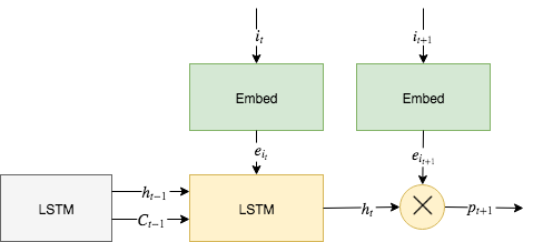
So given these ingredients, how do we now construct a sequential recommender? Let’s assume on every timestep \(t\in\{1,\ldots,T\}\) a user has interacted with an item \(i_t\). The basic idea is now to feed these interactions into an LSTM up to the time \(t\) in order to get a representation of the user’s preferences \(h_t\) and use that to state if the user might like or dislike the next item \(i_{t+1}\). Just like in a non-sequential recommender we also do a one-hot encoding of the items followed by an embedding into a dense vector representation \(e_{i_t}\) which is then feed into the LSTM. We can then just use the output \(h_t\) of the LSTM and calculate the inner product (\(\bigotimes\)) with the embedding \(e_{i_{t+1}}\) plus an item bias for varying item popularity to retrieve an output \(p_{t+1}\). This output along with others is then used to calculate the actual loss depending on our sample strategy and loss function. We train our model by sampling positive interactions and corresponding negative interactions. In an explicit feedback context a positive and negative interaction might be a positive and negative rating of a user for an item, respectively. In an implicit feedback context, all item interactions of a user are considered positive whereas negative interactions arise from items the user did not interact with. During the training we adapt the weights of our model so that for a given user the scalar output of a positive interaction is greater than the output of a negative interaction. This can be seen as an approximation to a softmax in very high-dimensional output space.
Figure 1 illustrates our sequential recommender model and this is what’s actually happening inside Spotlight’s sequential recommender with an LSTM representation. If you raise your eyebrow due to the usage of an inner product then be aware that low-rank approximations have been and still are one of the most successful building blocks of recommender systems. An alternative would be to replace the inner product with a deep feed forward network but to quite some extent, this would also just learn to perform an approximation of an inner product. A recent paper Latent Cross: Making Use of Context in Recurrent Recommender Systems by Google also emphasizes the power of learning low-rank relations with the help of inner products.
What we want to do is basically replacing the LSTM part of Spotlight’s sequential recommender with an mLSTM. But before we do that the obvious question is why? Let’s recap the formulae of a typical LSTM implementation like the one in PyTorch:
where \(i_t\) denotes the input gate, \(f_t\) the forget gate and \(o_t\) the output gate at timestep \(t\). If we look at those lines again we can see a lot of terms in the form of \(W_{**} x_t + W_{**} h_{t-1}\) neglecting the biases \(b_*\) for a moment. Thus a lot of an LSTM’s inner workings depend on the addition of the transformed input with the transformed hidden state. So what happens if a trained LSTM with thus fixed \(W_{**}\) encounters some unexpected, completely surprising input \(x_t\)? This might disturb the cell state \(c_t\) leading to pertubated future \(h_t\) and it might take a long time for the LSTM to recover from that singular surprising input. The authors of the paper Multiplicative LSTM for sequence modelling now argue that “RNN architectures with hidden-to-hidden transition functions that are input-dependent are better suited to recover from surprising inputs”. By allowing the hidden state to react flexibly on the new input by changing its magnitude it might be able to recover from mistakes faster. The quite vague formulation of input-dependent transition functions is then actually achieved in a quite simple way. In an mLSTM the hidden state \(h_{t-1}\) is transformed in a multiplicative way using the input \(x_t\) into an intermediate state \(m_t\) before it is used in a plain LSTM as before. Eventually, there is only a single equation to be prepended to the equations of an LSTM:
The element-wise multiplication (\(\odot\)) allows \(m_t\) to flexibly change it’s value with respect to \(h_{t-1}\) and \(x_t\). On a more theoretical note, if you picture the hidden states of an LSTM as a tree depending on the inputs at each timestep then the number of all possible states at timestep \(t\) will be much larger for an mLSTM compared to an LSTM. Therefore, the tree of an mLSTM will be much wider and consequently more flexible to represent different probability distributions according to the paper. The paper focuses only on NLP tasks but since surprising inputs are also a concern in sequential recommender systems, the self-evident idea is to evaluate if mLSTMs also excel in recommender tasks.
Implementation
Everyone seems to love PyTorch for it’s beautiful API and I totally agree. For me its beauty lies in its simplicity.
Every elementary building block of a neural network like a linear transformation is called a Module in PyTorch. A
Module is just a class that inherits from Module and implements a forward method that does the transformation
with the help of tensor operations. A more complex neural network is again just a Module and uses the
composition principle to compose its functionality from simpler modules. Therefore, in my humble opinion, PyTorch
found a much nicer concept of combining low-level tensor operations with the high level composition of layers compared
to core TensorFlow and Keras where you are either stuck on the level of tensor operations or the composition of layers.
For our task, we gonna need an mLSTM module and luckily PyTorch provides RNNBase, a base class for custom RNNs.
So all we have to do is to write a module that inherits from RNNBase, defines additional parameters and implements
the mLSTM equations inside of forward:
import math

import torch
from torch.nn import Parameter
from torch.nn.modules.rnn import RNNBase, LSTMCell
from torch.nn import functional as F


class mLSTM(RNNBase):
    def __init__(self, input_size, hidden_size, bias=True):
        super(mLSTM, self).__init__(
            mode='LSTM', input_size=input_size, hidden_size=hidden_size,
                 num_layers=1, bias=bias, batch_first=True,
                 dropout=0, bidirectional=False)

        w_im = torch.Tensor(hidden_size, input_size)
        w_hm = torch.Tensor(hidden_size, hidden_size)
        b_im = torch.Tensor(hidden_size)
        b_hm = torch.Tensor(hidden_size)
        self.w_im = Parameter(w_im)
        self.b_im = Parameter(b_im)
        self.w_hm = Parameter(w_hm)
        self.b_hm = Parameter(b_hm)

        self.lstm_cell = LSTMCell(input_size, hidden_size, bias)
        self.reset_parameters()

    def reset_parameters(self):
        stdv = 1.0 / math.sqrt(self.hidden_size)
        for weight in self.parameters():
            weight.data.uniform_(-stdv, stdv)

    def forward(self, input, hx):
        n_batch, n_seq, n_feat = input.size()

        hx, cx = hx
        steps = [cx.unsqueeze(1)]
        for seq in range(n_seq):
            mx = F.linear(input[:, seq, :], self.w_im, self.b_im) * F.linear(hx, self.w_hm, self.b_hm)
            hx = (mx, cx)
            hx, cx = self.lstm_cell(input[:, seq, :], hx)
            steps.append(cx.unsqueeze(1))

        return torch.cat(steps, dim=1)
The code is pretty much self-explanatory. We inherit from RNNBase and initialize the additional parameters we need for the calculation of \(m_t\)
in __init__. In forward we use those parameters to calculate \(m_t = (W_{im} x_t + b_{im}) \odot{} ( W_{hm} h_{t-1} + b_{hm})\) with the help of F.linear and pass it to an ordinary LSTMCell. We collect the results for each timestep
in our sequence in steps and return it as concatenated tensor.
The Spotlight library, in the spirit of PyTorch, also follows a modular concept of components that can be easily plugged together and replaced. It has only five components:
- embedding layers which map item ids to dense vectors,
- user/item representations which take embedding layers to calculate latent representations and the score for a user/item pair,
- interactions which give easy access to the user/item interactions and their explicit/implicit feedback,
- losses which define the objective for the recommendation task,
- models which take user/item representations, the user/item interactions and a given loss to train the network.
Due to this modular layout, we only need to write a new user/item representation module called mLSTMNet. Since this
is straight-forward I leave it to you to take a look at the source code in my mlstm4reco repository.
At this point I should mentioned that the whole layout of the repository was strongly inspired by Maciej Kula’s
Mixture-of-tastes Models for Representing Users with Diverse Interests paper and the accompanying source code.
My implementation also follows his advise of using an automatic hyperparameter optimisation for my own model and the
baseline model for comparison. This avoids quite a common bias in research when people put more effort in hand-tuning
their own model compared to the baseline to later show a better improvement in order to get the paper accepted.
Using a tool like HyperOpt for hyperparameter optimisation is quite easy and mitigates this bias to some extent at least.
Evaluation
To compare Spotlight’s ImplicitSequenceModel with an LSTM to an mLSTM user representation, the
mlstm4reco repository provides a run.py script in the experiments folder which takes several
command line options. Some might argue that this is a bit of over-engineering for a one time evaluation.
But for me it’s just one aspect of proper and reproducible research since it avoids errors and you can also easily
log which parameters were used to generate the results. I also used PyScaffold to set up proper Python package
scaffold within seconds. This allows me to properly install the mlstm4reco package and import its functionality from
wherever I want without messing around with the PYTHONPATH environment variable which one should never do anyway.
For the evaluation matrix below I ran each experiment 200 times to give HyperOpt enough chances to find good
hyperparameters for the number of epochs (n_iter), number of embeddings (embedding_dim), l2-regularisation (l2),
batch size (batch_size) and learning rate (learn_rate).
Each of our two models, i.e. lstm and mlstm user representation, were applied to three datasets,
the MovieLens 1m and 10m datasets as well as the Amazon dataset. For instance, to run 200 experiments with the mlstm
model on the Movielens 10m dataset the command would be ./run.py -m mlstm -n 200 10m.
In each experiment the data is split into a training, validation and test set where training is used to fit the model, validation to find the right hyperparameters and test for the final evaluation after all parameters are determined. The performance of the models is measured with the help of the mean reciprocal rank (MRR) score. Here are the results:
| dataset | type | validation | test | learn_rate | batch_size | embedding_dim | l2 | n_iter |
|---|---|---|---|---|---|---|---|---|
| Movielens 1m | LSTM | 0.1199 | 0.1317 | 1.93e-2 | 208 | 112 | 6.01e-06 | 50 |
| Movielens 1m | mLSTM | 0.1275 | 0.1386 | 1.25e-2 | 240 | 120 | 5.90e-06 | 40 |
| Movielens 10m | LSTM | 0.1090 | 0.1033 | 4.19e-3 | 224 | 120 | 2.43e-07 | 50 |
| Movielens 10m | mLSTM | 0.1142 | 0.1115 | 4.50e-3 | 224 | 128 | 1.12e-06 | 45 |
| Amazon | LSTM | 0.2629 | 0.2642 | 2.85e-3 | 224 | 128 | 2.42e-11 | 50 |
| Amazon | mLSTM | 0.3061 | 0.3123 | 2.48e-3 | 144 | 120 | 4.53e-11 | 50 |
If we compare the test results of the Movielens 1m dataset, it’s an improvement of 5.30% when using mLSTM over LSTM representation, for Movielens 10m it’s 7.96% more and for Amazon it’s even 18.19% more.
Conclusion
The performance improvements of using an mLSTM over an LSTM user representation are quite good but nothing spectacular. They give us at least some indication that mLSTMs achieve superior results for sequential recommendation tasks. In order to further underpin this first assessment one could test with more datasets and also check other evaluation metrics besides MRR. I leave this to a dedicated reader, so if you are interested, please let me know and share your results. With regard to my initial motivation and tasks, I have achieved much deeper insights into the domain of sequential recommenders and with the help of PyTorch, Spotlight I am looking forward to my next side project! Let me know if you liked this post and comment below.
Comments
comments powered by Disqus