Finally! Bayesian Hierarchical Modelling at Scale

Introduction

Since the advent of deep learning, everything is or has to be about Artificial Intelligence, so it seems. Even software which is applying traditional techniques from e.g. instrumentation and control engineering, is nowadays considered AI. For instance, the famous robots of Boston Dynamics are not based on deep reinforcement learning as many people think but much more traditional engineering methods. This hype around AI, which is very often equated with deep learning, seems to draw that much attention such that great advances of more traditional methods seem to go almost completely unnoticed. In this blog post, I want to draw your attention to the somewhat dusty Bayesian Hierarchical Modelling. Modern techniques and frameworks allow you to finally apply this cool method on datasets with sizes much bigger than what was possible before and thus letting it really shine.

So for starters, what is Bayesian Hierarchical Modelling and why should I care? I assume you already have a basic knowledge about Bayesian inference, otherwise Probabilistic Programming and Bayesian Methods for Hackers is a really good starting point to explore the Bayesian rabbit hole. In simple words, Bayesian inference allows you to define a model with the help of probability distributions and also incorporate your prior knowledge about the parameters of your model. This leads to a directed acyclic graphical model (aka Bayesian network) which is explainable, visual and easy to reason about. But that’s not even everything, you also get Uncertainty Quantification for free, meaning that the model’s parameters are not mere point estimates but whole distributions telling you how certain you are about their values.

A classical statistical method that most data scientists learn about early on is linear regression. It can also be interpreted in a Bayesian way giving you the possibility to define prior knowledge about the parameters, e.g. that they have to be close to zero or that they are non-negative. Then again, many of the priors you might come up with could also be seen as mere regularizers in a non-Bayesian way, and treated like that, often efficient techniques exist to solve such formulations. So where the Bayesian framework now really shines is, if you consider the following problem setting I stole from the wonderful presentation A Bayesian Workflow with PyMC and ArviZ by Corrie Bartelheimer.

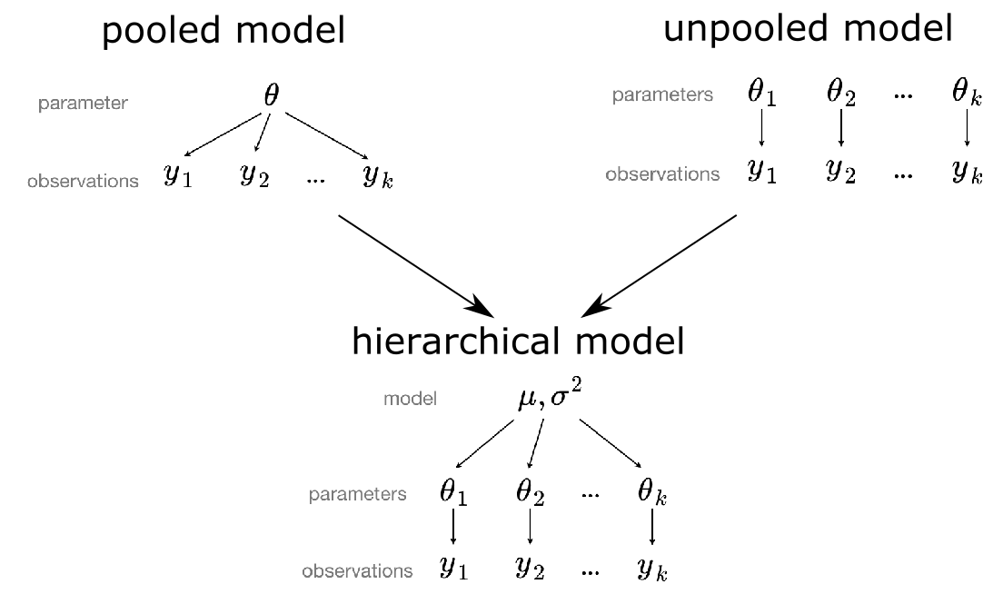
Imagine you want to estimate the price of an apartment in Berlin given its living area in square meters and district. Making a linear regression with all data points you have neglecting the districts, i.e. a pooled model, will lead to a robust estimation of the slope and intercept but a wide residual distribution. This is due to the fact that the price of an apartment also heavily depends on the district it is located in. Now grouping your data with respect to the respective districts and making a linear regression for each, i.e. an unpooled model, will lead to a much more narrow residual distribution but also a high uncertainty in your parameters since some district might only have three data points. To combine the advantages of a pooled and unpooled model, one would intuitively demand that for each district the prior knowledge of the parameter from the pooled model should be used and updated according to the data we have about a certain district. If we have only a few data points we would only allow to deviate a bit from our prior knowledge about the parameter. In case we have lots of data points, the parameter for the respective district should be allowed to have a huge difference compared to the parameter of the pooled model. Thus the pooled model acts as an informed prior for the parameters within the unpooled model leading altogether to an hierarchical model, which is sometimes also referred to as partially pooled model. Figure 1 illustrates our thoughts so far.

Recent Advances

So far I mostly used PyMC3 for Bayesian inference or probabilistic programming as the authors of PyMC3 like to call it. I love it for it’s elegant design and consequently its expressiveness. The documentation is great and thus you can pretty much hack away with your model ideas. The only problem I always had with it is that for me it never scaled so well with somewhat larger datasets, i.e. more than 100k data points, and a larger number of parameters. There is a technical and methodical reason for it. Regarding the former, PyMC3 uses Theano to speed up its computations by transpiling your Python code to C. Theano inspired many frameworks like Tensorflow and PyTorch but is considered deprecated today and cannot rival the speed of modern frameworks anymore. For the latter, I used PyMC3 mostly with Markov chain Monte Carlo (MCMC) based methods, which are sampling algorithms and thus computationally quite demanding, while variational inference (VI) methods are much faster. But also when using VI, which PyMC3 also supports, it never really allowed me to deal with larger datasets rendering Bayesian Hierarchical Modelling (BHM) a wonderful tool that sadly could not be applied in many suitable projects due to its computational costs.

Luckily, the world of data science moves on with an incredible speed, and some time ago I had a nice project at my hand that could make good use of BHM. Thus, I gave it another shot and also looked beyond PyMC3. My first candidate to evaluate was Pyro, which uses Stochastic Variational Inference (SVI) by default, and calls itself a deep universal probabilistic programming framework. Instead of Theano it is based on PyTorch and thus allows for just-in-time (JIT) compilation, which sped up my test case already quite a bit. Pyro also emphasizes vectorization, thus allowing for fast parallel computation, e.g. SIMD operations. In total the speed-up compared to PyMC3 was amazing in my test-case letting me almost forget the two downsides of Pyro compared to PyMC3. Firstly, the documentation of Pyro is not as polished and secondly, it’s just so much more complicated to use and understand but your mileage may vary on that one.

Digging through the website of Pyro I then stumbled over NumPyro that has a similar interface compared to Pyro but uses JAX instead of PyTorch as its backend. JAX is like NumPy on steroids. It’s crazy fast as it uses XLA, which is a domain-specific compiler for linear algebra operations. Additionally, it allows for automatic differentiation like Autograd, whose maintainers moved over to develop JAX further. Long story short, NumPyro even blew the benchmark results of Pyro out of the water. For the first time (at least for what I know), NumPyro allows you do Bayesian inference with lots of parameters like in BHM on large data! In the rest of this post, I want to show you how NumPyro can be applied in a typical demand prediction use-case on some public dataset. The dataset in my actual use-case was much bigger, my model had more parameters and NumPyro could still handle it but you just have to trust me on this one ;-) Hopefully some readers will find this post useful and maybe it mitigates a bit the pain coming from the lack of NumPyro’s documentation and examples.

Use-Case & Modelling

Imagine you have many retail stores and want to make individual demand predictions for them. For stores that were opened a long time ago, this should be no problem but how do you deal with stores that first opened a week ago or even will open soon? Like in the example of apartment prices in different districts, BHM helps you to deal exactly with this cold start problem. We take the Rossmann dataset from Kaggle to simulate this problem by removing the data of some of the stores. The data consists of a train dataset with information about the sales and daily features of the stores, e.g. if a promotion happened (promo), as well as a store dataset with time-independent store features. Here’s what we wanna do in our little experiment and study protocol:

1. join the data from Kaggle’s train.csv dataset with the general store features from the store.csv dataset,
2. perform some really basic feature engineering and encoding of the categorical features,
3. split the data into train and test where we treat the stores from train as being opened for a long time and the ones from test as newly opened,
4. fit our hierarchical model on the train dataset to infer the “global” parameters of the upper model hierarchy,
5. take only the first 7 days for each store in the test data, which we assume to know, and fit our model only inferring the local, i.e. store-specific, parameters of the lower hierarchy while keeping the global ones fixed,
6. compare the inferred parameters of a test store to:
   1. the inferred local parameters of a simple Poisson model. We expect them to be completely different due to the lack of data and thus overfitting of the Poisson model,
   2. the inferred local parameters of our model if we had given it the whole time series from test, i.e. not only the first 7 days. In this case, we assume that we are already pretty close since the priors given by the global parameters nudge them in the right direction even with only little data.

All code of this little experiment can be found under my bhm-at-scale repository so that you can follow along easily. The steps 1-3 are performed in the preprocessing notebook and are actually not that interesting, thus we will skip it here. Steps 4-6 are performed in the model notebook while some visualisations are presented in the evaluation notebook.

But before we start to get technical, let’s take a minute and frame again the forecasting problem from a more mathematical side. The data of each store is a time-series of feature vectors and target scalars. We want to find a mapping such that the feature vector of each time-step is mapped to a value close to the target scalar of the respective time-step. Since our target value, i.e. the number of sales, is a non-negative integer we could assume a Poisson distribution and consequently perform a Poisson regression in a hierarchical way. This would be kind of okay if we were only interested in a point estimation and thus would not care about the variance of the predictive posterior distribution. The Poisson distribution only has one parameter \(\lambda\) that allows you to define the mean \(\mu\) while the variance \(\sigma^2\) then just equals the mean as there is no way to adjust the variance independently.
In many practical use-cases, there is overdispersion though, meaning that the variance is larger than the mean and we have to make up for it. We can define a so called dispersion parameter \(r\in(0,\infty)\) by reparametrization in the negative binomial distribution, i.e.

where \(\Gamma\) is the Gamma function. Now we have

and using \(r\) we are thus able to adjust the variance from \(\mu\) to \(\infty\). Another name for the negative binomial distribution is Gamma-Poisson distribution and this is the name under which we find it also in NumPyro. I find this name much more catchy since you can imagine a Poisson distribution with its only parameter drawn from a Gamma distribution that has two parameters \(\alpha\) and \(\beta\). This also intuitively explains why the variance of NB is bounded below by its mean. Just think of NB as a generalization of the Poisson distribution with one more parameter that allows adjusting the variance.

Uncertainty Quantification is a crucial requirement for demand forecasts in retail although peculiarly, no one really cares about forecasts in retail anyway. What retailers really care about is optimal replenishment, meaning that they want to have a system telling them how much to order so that there is an optimal amount of stocks available in their store. In order to provide optimal replenishment suggestions you need demand forecasts that provide probability distributions, not only point estimations. With the help of those distributions the replenishment system basically runs an optimization with respect to some cost function, e.g. cost of a missed sale is weighted 3 times the cost of a written-off product, and further constraints, e.g. if products can only be ordered in bundles of 10. For these reasons we will use the NB distribution that allows us the quantify the uncertainties in our sales predictions adequately.

So now that we settled with NB as the distribution that we want to fit to the daily sales of our stores \(\mathbf{y}\), we can think about incorporating our features \(\mathbf{x}\). We want to use a linear model to map \(\mathbf{x}\) to \(\mathbf{\mu}\) such that we can use it later to calculate \(\alpha\) and \(\beta\) of NB. Using again the fact that we are dealing with non-negative numbers and also considering that we expect effects to be multiplicative, e.g. 10% more during a promotion, our ansatz is

where \(\mathbf{\theta}\) is a vector of coefficients. For each store \(i\) and each feature \(j\) we will have a separate coefficient \(\theta_{ij}\). The \(\theta_{ij}\) are regularized by parameters \(\theta^\mu_j\) and \(\theta^{\sigma^2}_j\) on the global level, which helps us in case a store has only little historical data. For the dispersion parameters we infer individual \(r_i\) for each store \(i\) as well as global parameters \(r^\mu\) and \(r^{\sigma^2}\) over all stores. And that’s already most of it. Figure 2 depicts the graphical model outlined so far.

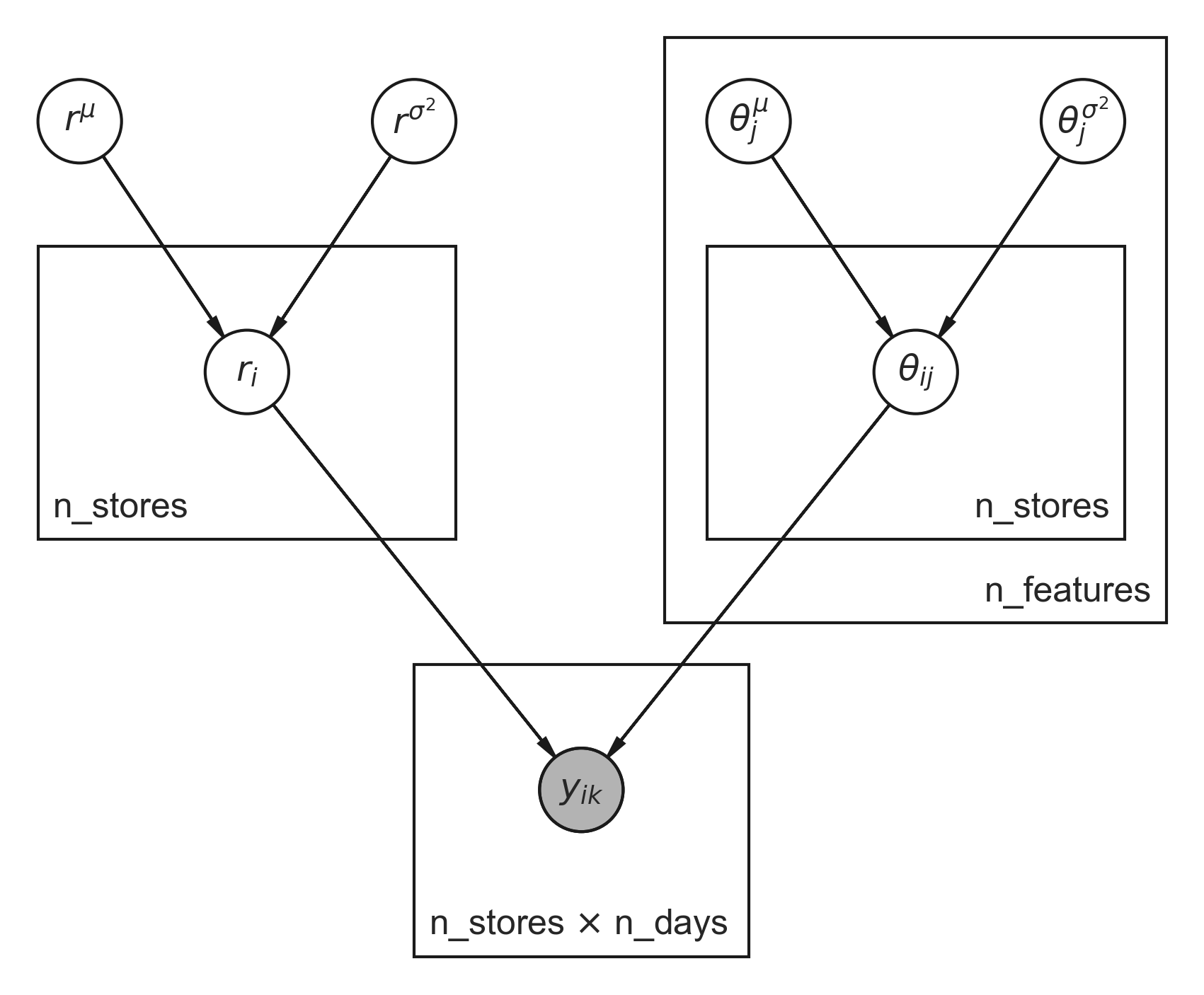
Those boxes in Figure 2, which are called plates, tell you how many times a parameter is repeated. Nested plates are multiplied by the number given by outer plates, which can also be seen by looking at the number of indices. The concept of plates was also taken up by the authors of NumPyro to express that certain dimensions are conditionally independent. This also helps them to increase performance by taking optimizations into account that are just not possible in the general case. Shaded circles are observed values, which in our case are the number of sales on a given day \(k\) and store \(i\).

Implementation

Let’s take a quick look into our model code which is just a normal Python function. It’s good to keep in mind, that we call this a model since we assume that given the right parameters it would be able to generate sales for some given stores and days resembling the observed sales for these stores and days. The model function only defines the model parameters, how they interact and their priors.

import numpyro
import numpyro.distributions as dist
from numpyro.infer.reparam import TransformReparam
from jax.numpy import DeviceArray
import jax.numpy as jnp
from jax import random


def model(X: DeviceArray) -> DeviceArray:
    """Gamma-Poisson hierarchical model for daily sales forecasting

    Args:
        X: input data

    Returns:
        output data
    """
    n_stores, n_days, n_features = X.shape
    n_features -= 1  # remove one dim for target
    eps = 1e-12  # epsilon

    plate_features = numpyro.plate("features", n_features, dim=-1)
    plate_stores = numpyro.plate("stores", n_stores, dim=-2)
    plate_days = numpyro.plate("timesteps", n_days, dim=-1)

    disp_param_mu = numpyro.sample(
        "disp_param_mu",
        dist.Normal(loc=4., scale=1.)
    )
    disp_param_sigma = numpyro.sample(
        "disp_param_sigma",
        dist.HalfNormal(scale=1.)
    )

    with plate_stores:
        with numpyro.handlers.reparam(config={"disp_params": TransformReparam()}):
            disp_params = numpyro.sample(
                "disp_params",
                dist.TransformedDistribution(
                    dist.Normal(loc=jnp.zeros((n_stores, 1)), scale=0.1),
                    dist.transforms.AffineTransform(disp_param_mu, disp_param_sigma),
                ),
            )

    with plate_features:
        coef_mus = numpyro.sample(
            "coef_mus",
            dist.Normal(loc=jnp.zeros(n_features),
                        scale=jnp.ones(n_features))
        )
        coef_sigmas = numpyro.sample(
            "coef_sigmas",
            dist.HalfNormal(scale=2.*jnp.ones(n_features))
        )

        with plate_stores:
            with numpyro.handlers.reparam(config={"coefs": TransformReparam()}):
                coefs = numpyro.sample(
                    "coefs",
                    dist.TransformedDistribution(
                        dist.Normal(loc=jnp.zeros((n_stores, n_features)), scale=1.0),
                        dist.transforms.AffineTransform(coef_mus, coef_sigmas),
                    ),
                )

    with plate_days, plate_stores:
        targets = X[..., -1]
        features = jnp.nan_to_num(X[..., :-1])  # padded features to 0
        is_observed = jnp.where(jnp.isnan(targets), jnp.zeros_like(targets), jnp.ones_like(targets))
        not_observed = 1 - is_observed
        means = (is_observed * jnp.exp(jnp.sum(jnp.expand_dims(coefs, axis=1) * features, axis=2))
                 + not_observed*eps)

        betas = is_observed*jnp.exp(-disp_params) + not_observed
        alphas = means * betas
        return numpyro.sample("days", dist.GammaPoisson(alphas, betas), obs=jnp.nan_to_num(targets))

Note that disp_param is \(r\) and coef is \(\theta\) in the source code above for better readability. You will recognize a lot of what we have talked about and I don’t want to go into the syntactical details of NumPyro. My suggestion would be to first read the documentation of Pyro, as it is way more comprehensive, and then look up the differences in the NumPyro reference.

Reading the source code more thoroughly, you might wonder about the definition of the coefficients as:

with numpyro.handlers.reparam(config={"coefs": TransformReparam()}):
    coefs = numpyro.sample(
        "coefs",
        dist.TransformedDistribution(
            dist.Normal(loc=jnp.zeros((n_stores, n_features)), scale=1.0),
            dist.transforms.AffineTransform(coef_mus, coef_sigmas),
        ),
    )

The explanations of the model I have given and also the plot, actually shows the centered version of a hierarchical model. For me the centered version feels much more intuitive and is easier to explain. The downside is that the direct dependency of the local parameters on the global ones make it hard for many MCMC sampling methods but also SVI methods to explore certain regions of the local parameter space. This effect is called funnel and can be imagined as walking with the the same step length on a bridge that gets narrower and narrower. From the point on where the bridge is about as wide as your step length, you might become a bit hesitant to explore more of it. As very often the case, a reparameterization overcomes this problem resulting in the non-centered version of a hierarchical model. This is the version used in the implementation. If you want to know more about this, a really great blog post by Thomas Wiecki gives you all the details about it.

Another thing that wasn’t mentioned yet are the is_observed and not_observed variables which are just a nice gimmick. Instead of using up degrees of freedom to learn that the number of sales is 0 on days where the store is closed, I set the target variable \(y\) to not observed instead of 0. During training, these target values are just ignored and later allows the model to answer a store manager’s potential question: “How many sales would I have had if I had opened my store on that day?”

Until now we have talked about the model and if you are a PyMC3 user, you might think that this should be enough to actually solve it. Pyro and NumPyro have a curious difference with respect to that. To actually fit the parameters of the model, distributions for the parameters have to be defined since its SVI. This is done in a separate function called guide.

def guide(X: DeviceArray):
    """Guide with parameters of the posterior

    Args:
        X: input data
    """
    n_stores, n_days, n_features = X.shape
    n_features -= 1  # remove one dim for target

    plate_features = numpyro.plate("features", n_features, dim=-1)
    plate_stores = numpyro.plate("stores", n_stores, dim=-2)

    disp_param_mu = numpyro.sample(
        "disp_param_mu",
        dist.Normal(loc=numpyro.param("loc_disp_param_mu", 4.*jnp.ones(1)),
                    scale=numpyro.param("scale_disp_param_mu", 1.*jnp.ones(1),
                                        constraint=dist.constraints.positive))
    )
    disp_param_sigma = numpyro.sample(
        "disp_param_sigma",
        dist.TransformedDistribution(
            dist.Normal(loc=numpyro.param("loc_disp_param_logsigma", 1.0*jnp.ones(1)),
                        scale=numpyro.param("scale_disp_param_logsigma", 0.1*jnp.ones(1),
                                            constraint=dist.constraints.positive)),
            transforms=dist.transforms.ExpTransform())
    )

    with plate_stores:
        with numpyro.handlers.reparam(config={"disp_params": TransformReparam()}):
            numpyro.sample(
                "disp_params",
                dist.TransformedDistribution(
                    dist.Normal(
                        loc=numpyro.param("loc_disp_params", jnp.zeros((n_stores, 1))),
                        scale=numpyro.param("scale_disp_params", 0.1 * jnp.ones((n_stores, 1)),
                                            constraint=dist.constraints.positive,
                        ),
                    ),
                    dist.transforms.AffineTransform(disp_param_mu, disp_param_sigma),
                ),
            )

    with plate_features:
        numpyro.sample(
            "coef_mus",
            dist.Normal(loc=numpyro.param("loc_coef_mus", jnp.ones(n_features)),
                        scale=numpyro.param("scale_coef_mus", 0.5*jnp.ones(n_features),
                                            constraint=dist.constraints.positive))
        )
        numpyro.sample(
            "coef_sigmas",
            dist.TransformedDistribution(
                dist.Normal(loc=numpyro.param("loc_coef_logsigmas", jnp.zeros(n_features)),
                            scale=numpyro.param("scale_coef_logsigmas", 0.5*jnp.ones(n_features),
                                                constraint=dist.constraints.positive)),
                transforms=dist.transforms.ExpTransform())
        )

        with plate_stores:
            with numpyro.handlers.reparam(config={"coefs": TransformReparam()}):
                numpyro.sample(
                    "coefs",
                    dist.TransformedDistribution(
                        dist.Normal(
                            loc=numpyro.param("loc_coefs", jnp.zeros((n_stores, n_features))),
                            scale=numpyro.param("scale_coefs", 0.5 * jnp.ones((n_stores, n_features)),
                                                constraint=dist.constraints.positive,
                            ),
                        ),
                        dist.transforms.AffineTransform(coef_mus, coef_sigmas),
                    ),
                )

As you can see, the structure of the guide reflects the structure of the model and there we are just defining for each model parameter a distribution that again has parameters that need to be determined. The link between model and guide is given by the names of the sample sites like “coef_offsets”. This is a bit dangerous as a single typo in the model or guide may break this link leading to unexpected behaviour. I spent more than a day of debugging a model once until I realized that some sample site in the guide had a typo. You can see in the actual implementation, i.e. model.py, that I learnt from my mistakes as this source of error can be completely eliminated by simply defining class variables like:

class Site:
    disp_param_mu = "disp_param_mu"
    disp_param_sigma = "disp_param_sigma"
    disp_param_offsets = "disp_param_offsets"
    disp_params = "disp_params"
    coef_mus = "coef_mus"
    coef_sigmas = "coef_sigmas"
    coef_offsets = "coef_offsets"
    coefs = "coefs"
    days = "days"

Then using variables like Site.coef_offsets instead of strings like "coef_offsets" as identifiers of sample sites, allows your IDE to inform you about any typo as you go. Problem solved.

Besides the model and guide, we also have to define a local guide and a predictive model. The local guide assumes that we have already fitted the global parameters but want to only determine the local parameters of new stores with little data. The predictive model assumes global and local parameters to be already inferred so that we can use it to predict the number of sales on days beyond our training interval. As these functions are only slide variations, I spare you the details and refer you to the implementation in model.py.

Most parts of the model notebook actually deal with training the model on stores from the training data with a long sales history, then fixing the global parameters and fitting the local guide on the stores from the test set with a really short history of 7 days. This works really well although the number of features, which is 23, is much higher than 7! Let’s take a look at the coefficients of a store from the test set as detailed in the model notebook:

[ 2.7901888   2.6591218   2.6881874   2.6126788   2.656775    2.554397
  2.4938385   0.33227605  3.115691    2.9264386   2.692092    2.9548435
  0.05613964  0.06542112  2.8379264   2.9023972   3.5701406   3.2074358
  4.0569873   2.9304545   2.7463424   2.823191    2.959007  ]

The notebook also shows that the traditional Poisson regression using Scikit-Learn overfits the training set and yields implausible coefficients. Comparing the coefficients from above to the ones of the Poisson regression for the same store, i.e.

[ 1.1747563  -2.2386415   2.1442924   1.9889396   1.9385103   1.8024149
 -6.8102717   1.1747563   2.2386413  -2.2386413   0.          0.
 -0.09434899  0.          0.          0.          0.          0.
  0.          0.          0.          0.          0.        ]

we see that they are highly different and zero for features in the Poisson regression that weren’t encountered in the data of just 7 days. Now comparing the coefficients of our BHM model trained on just 7 days with the coefficients of a cheating model trained on the whole test set, i.e.

[ 2.814997    2.7551868   2.6182172   2.6453698   2.672692    2.5201027
  2.593036    0.2265296   3.184446    3.1163387   2.5429602   2.9477317
 -0.03218627  0.06836608  2.8726482   2.925492    3.56679     3.215817
  4.0523443   2.9164758   2.7241356   2.8247747   2.9598234 ]

we see that they are quite similar. That’s the magic of a hierarchical model! We started with plausible defaults from a global perspective and adapted locally depending on the amount of available data.

Running the code from the model notebook on your laptop will be matter of a few minutes for the training on 1000 stores each having 942 days of sales and 23 features for each store and day. In total this leads to roughly one million data points and \(23\cdot 1000+1000+2\cdot 23+2=24048\) parameters in our graphical model. Since each parameter is fitted with the help of a parameterized distribution in the guide, as we are doing SVI, the number of actual variables is twice as much leading to roughly 50,000 variables that need to be fitted. While 50k parameters and about 1 Million data points surely is not big data, it’s still impressive that using NumPyro you can fit a model like that within a few minutes on your laptop and the implementation is not even using batching that would speed it up even further. In one of my customer projects we used a way larger model on much more data and our workstation was still able to handle it smoothly. NumPyro really scales well even beyond this little demonstration.

Visualization

There is now tons of things one could do with the results of our hierarchical model. One could check out the actual prediction results, look at how certain we are about the parameters like the coefficients and so on. Most of that I will leave to the interested reader and give only a few tidbits here from the evaluation notebook. We start with taking a look at the sales prediction for one of the stores from the test set as depicted in Figure 3.

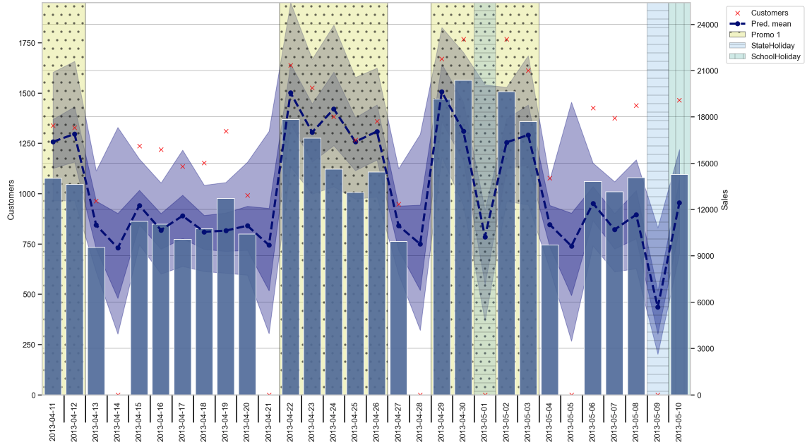
Only judging by the eye, we see that predicted mean (blue dashed line) follows the number of sales (bluish bars) quite good. The background is shaded according to some important features like promotions and holidays which explain some of the variations in our predictions. Just for information, also the number of customers are displayed but not used in the prediction of course. Also, we see the 50% and 90% credible intervals as shaded blue areas around our mean, which tell us how certain we are about our predictions. We can also see that on Sundays, when the store was closed, we predict not 0 but what would have likely happened if it wasn’t closed, which was part of our model.

We could then also start looking into the effects of certain features like the weekdays. Figure 4 shows for each weekday starting with Monday a density over the means of all stores.

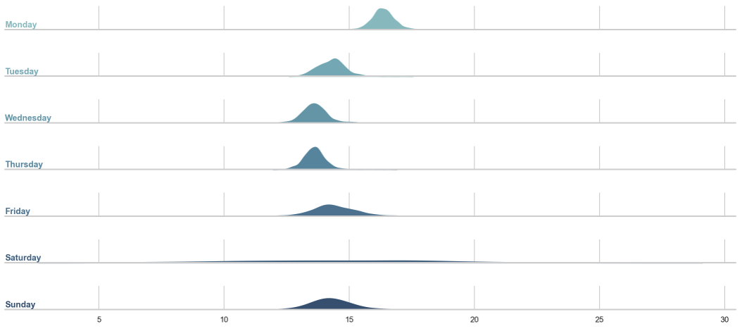
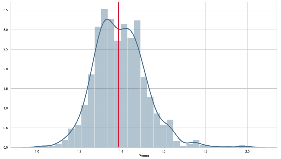
We can see that on average there seem to be a higher sales uplift on Mondays and also a high variance for the means on Saturdays and Sundays when many stores are closed. If we are more interested in things we can change, like when to do a promotion, we could be interested in analyzing the distribution of the promotion effect over all stores as shown in Figure 5.

These are just some analysis one could start to look into to derive useful insights for store management. The rest is up to your imagination and also depending on your use-case. Imagine we had a dataset that features not only the aggregated sales but also the ones of individual products, i.e. SKU-level. We could then build hierarchies over the product hierarchies and thus addressing cannibalization effects, e.g. when we introduce a new type of wine within our current offering. We could also use BHM to address censored data, which is also an important task when doing demand forecasts. So far we have used the words sales forecast and demand forecast interchangeably but bear in mind that we are actually interested in the demand. Canonically, one assumes that the demand for a product equals its sales but this only holds true if there was no out-of-stock situation in which we only know that demand ≥ sales. Right-censored data like that provides us with information about the cumulative distribution function in contrast to the probability mass function in case of no out-of-stock situation. There are ways to include both types of information into a BHM. Those are just some of many possible improvements and extensions to this model. I am looking forward to your ideas and use-cases!

Final Remarks

We have seen that BHM allows us to combine the advantages of a pooled and unpooled model. Using some retailer’s data, we implemented a simple BHM thereby also outlining the advantages of a Bayesian approach like uncertainty quantification and explainability. From a practical perspective, we have seen that BHM even scales really well with the help of NumPyro. On the theoretical side, we have talked about the Poisson distribution and why we preferred the Gamma-Poisson distribution. Finally, I hope to have conveyed the most important point of this post well, being that these models can now be applied to practical dataset sizes with the help of NumPyro! Cheers to that and let’s follow a famous saying in the French world of mathematics Poisson sans boisson est poison!