Motivation
If you have ever done something analytical or anything closely related to data science in Python, there is just no way you have not heard of Jupyter or IPython notebooks. In a nutshell, a notebook is an interactive document displayed in your browser which contains source code, e.g. Python and R, as well as rich text elements like paragraphs, equations, figures, links, etc. This combination makes it extremely useful for explorative tasks where the source code, documentation and even visualisations of your analysis are strongly intertwined. Due to this unique characteristic, Jupyter notebooks have achieved a strong adoption particularly in the data science community. But as Pythagoras already noted “If there be light, then there is darkness.” and with Jupyter notebooks it’s no difference of course.
Being in the data science domain for quite some years, I have seen good but also a lot of ugly. Notebooks that are beautifully designed and perfectly convey ideas and concepts by having the perfect balance between text, code and visualisations like in my all time favourite Probabilistic Programming and Bayesian Methods for Hackers. In strong contrast to this, and actually more often to find in practise, are notebooks with cells containing pages of incomprehensible source code, distracting you from the actual analysis. Also sharing these notebooks is quite often an unnecessary pain. Notebooks that need you to tamper with the PYTHONPATH or to start Jupyter from a certain directory for modules to import correctly. In this blog post I will introduce several best practices and techniques that will help you to create notebooks which are focused, easy to comprehend and to work with.
History
Before we get into the actual subject let’s take some time to understand how Project Jupyter evolved and where it came from. This will also clarify the confusion people sometimes have over IPython, Jupyter and JupyterLab notebooks. In 2001 Fernando Pérez was quite dissatisfied with the capabilities of Python’s interactive prompt compared to the commercial notebook environments of Maple and Mathematica which he really liked. In order to improve upon this situation he laid the foundation for a notebook environment by building IPython (Interactive Python), a command shell for interactive computing. IPython quickly became a success as the REPL of choice for many users but it was only a small step towards a graphical interactive notebook environment. Several years and many failed attempts later, it took until late 2010 for Grain Granger and several others to develop a first graphical console, named QTConsole which was based on QT. As the speed of development picked up, IPython 0.12 was released only one year later in December 2011 and included for the first time a browser-based IPython notebook environment. People were psyched about the possibilities IPython notebook provided them and the adoption rose quickly.
In 2014, Project Jupyter started as a spin-off project from IPython for several reasons. At that time IPython encompassed an interactive shell, the notebook server, the QT console and other parts in a single repository with the obvious organisational downsides. After the spin-off, IPython concentrated on providing solely an interactive shell for Python while Project Jupyter itself started as an umbrella organisation for several components like Jupyter notebook and QTConsole, which were moved over from IPython, as well as many others. Another reason for the split was the fact that Jupyter wanted to support other languages besides Python like R, Julia and more. The name Jupyter itself was chosen to reflect the fact that the three most popular languages in data science are supported among others, thus Jupyter is actually an acronym for Julia, Python, R.
But evolution never stops and the source code of Jupyter notebook built on the web technologies of 2011 started to show its age. As the code grew bigger, people also started to realise that it actually is more than just a notebook. Some parts of it rather dealt with managing files, running notebooks and parallel workers. This eventually led again to the idea of splitting these functionalities and laid the foundation for JupyterLab. JupyterLab is an interactive development environment for working with notebooks, code and data. It has full support for Jupyter notebooks and enables you to use text editors, terminals, data file viewers, and other custom components side by side with notebooks in a tabbed work area. Since February 2018 it’s officially considered to be ready for users and the 1.0 release is expected to happen end of 2018.
According to my experience in the last months, JupyterLab is absolutely ready and I recommend everyone to migrate to it. In this post, I will thus focus on JupyterLab and the term notebook or sometimes even Jupyter notebook actually refers to a notebook that was opened with JupyterLab. Practically this means that you run jupyter lab instead of jupyter notebook. If you are interested in more historical details read the blog posts of Fernando Pérez and Karlijn Willems.
Preparation & Installation
The first good practice can actually be learnt before even starting JupyterLab. Since we want our analysis to be reproducible and shareable with colleagues it’s a good practice to create a clean, isolated environment for every task. For Python you got basically two options virtualenv (also descendants like pipenv) or conda to achieve this. My favorite is conda for several reasons. First of all conda is a package manager of the Anaconda distribution and allows you to install more than just Python packages. Anaconda is more like a whole operation system coming with packages for Python, R and C/C++ system libraries like libc. From this point of view it’s much more than what virtualenv provides, since conda will also install system libraries like glibc if need be. Also the Python interpreter itself is installed separately into an isolated environment and thus independent of the one provided by your system. This makes it possible to easily pin down even the Python version of your environment. The tool pyenv allows you to do the same within the virtualenv ecosystem but conda feels just more integrated and gives a unified approach. In total, conda allows for much more fined-grained control of what is going on in your virtual environment than virtualenv with less side effects induced by your system.
For these reasons conda is much more common than virtualenv in the field of data science, thus we will use it in this tutorial. Still, everything shown here can analogously be conducted with the help of virtualenv/pipenv and all the concepts still apply as is also illustrated in a blog post of Christopher Prohm. For this tutorial, I assume you have Miniconda installed on your system. Besides this, every programmer’s machine should have Git installed and set up. The result of the following demonstration can be found in the boston_housing repository.
0. Use an isolated environment
In the spirit of Phil Karlton who supposedly said “There are only two hard things in Computer Science: cache invalidation and naming things.”, we gonna select a specific task, namely an analysis based on the all familiar Boston housing dataset, to help us finding crisp names. Based on our task we create an environment boston_housing including Python and some common data science libraries with:
conda create -n boston_housing python=3.6 jupyterlab pandas scikit-learn seaborn
After less than a minute the environment is ready to be used and we can activate it with conda activate boston_housing.
Efficient Workflow
The code in notebooks tends to grow and grow to the point of being incomprehensible. To overcome this problem, the only way is to extract parts of it into Python modules once in a while. Since it only makes sense to extract functions and classes into Python modules, I often start cleaning up a messy notebook by thinking about the actual task a group of cells is accomplishing. This helps me to refactor those cells into a proper function which I can then migrate into a Python module.
At the point where you create custom modules, things get trickier. By default Python will only allow you to import modules that are installed in your environment or in your current working directory. Due to this behaviour many people start creating their custom modules in the directory holding their notebook. Since JupyterLab is nice enough to set the current working directory to the directory containing your notebook, everything is fine at the beginning. But as the number of notebooks that share common functionality imported from modules grows, the single directory containing notebooks and modules will get messier as you go. The obvious split of notebooks and modules into different folders or even organizing your notebooks into different folders will not work with this approach since then your imports will fail.
This observation brings us to one of the most important best practices: develop your code as a Python package. A Python package will allow you to structure your code nicely over several modules and even subpackages, you can easily create unit tests and the best part of it is that distributing and sharing it with your colleagues comes for free. But creating a Python package is so much overhead; surely it’s not worth this small little analysis I will complete in half a day anyway and then forget about it, I hear you say. Well, how often is this actually true? Things always start out small but then get bigger and messier if you don’t adhere to a certain structure right from the start. About half a year later then, your boss will ask you about that specific analysis you did back then and if you could repeat it with the new data and some additional KPIs. But more importantly coming back to the first part of your comment, if you know how, it’s no overhead at all!
1. Develop your code in a Python Package
With the help of PyScaffold it is possible to create a proper and standard-compliant Python package within a second. Just install it while having the conda environment activated with:
conda install -c conda-forge pyscaffold
This package adds the putup command into our environment which we use to create a Python package with:
putup boston_housing
Now we can change into the new boston_housing directory and install the package inside our environment in development mode:
python setup.py develop
The development mode installs the package in the conda environment by linking to the source code which resides in boston_housing/src/boston_housing. By doing so all your changes to the code will be directly available without any need to reinstall the package again.
Let’s start JupyterLab with jupyter lab from the root of your new project where setup.py resides. To keep everything tight and clean, we start by creating a new folder notebooks using the file browser in the left sidebar. Within this empty folder we create a new notebook using the launcher and rename it to housing_model. Within the notebook we can now directly test our package by typing:
from boston_housing.skeleton import fib
The skeleton module is just a test module that PyScaffold provides (omit it with putup --no-skeleton ...) and we import the Fibonacci function fib from it. You can now just test this function by calling fib(42) for instance.
At that point after having only adhered to a single good practice, we already benefit from many advantages. Since we have nicely separated our notebook from the actual implementation, we can package and distribute our code by just calling python setup.py bdist_wheel and use twine to upload it to some artefact store like PyPI or devpi for internal-only use. Another big plus is that having a package allows us to collaboratively work on the source code in your package using Git. On the other hand using Git with notebooks is a big pain since it its format is not really designed to be human-readable and thus merge conflicts are a horror.
Still we haven’t yet added any functionality, so let’s see how we do about that.
2. Extract functionality from the notebook
We start with loading the Boston housing dataset into a dataframe with columns of the lower-cased feature names and the target variable price:
import pandas as pd
from sklearn.datasets import load_boston

boston = load_boston()
df = pd.DataFrame(boston.data, columns=(c.lower() for c in boston.feature_names))
df['price'] = boston.target
Now imagine we would go on like this, do some preprocessing etc., and after a while we would have a pretty extensive notebook of statements and expressions without any structure leading to name collisions and confusion. Since notebooks allow the executing of cells in different order this can be extremely harmful. For these reasons, we create a function instead:
def get_boston_df():
    boston = load_boston()
    df = pd.DataFrame(boston.data, columns=(c.lower() for c in boston.feature_names))
    df['price'] = boston.target
    return df
We test it inside the notebook but then directly extract and move it into a module model.py that we create within our package under src/boston_boston. Now, inside our notebook, we can just import and use it:
from boston_housing.model import get_boston_df

df = get_boston_df()
Now that looks much cleaner and allows also for other notebooks to just use this bit of functionality without using copy & paste! This leads us to another best practice: Use JupyterLab only for integrating code from your package and keep complex functionality inside the package. Thus, extract larger bits of code from a notebook and move it into a package or directly develop code in a proper IDE.
3. Use a proper IDE
At that point the natural question comes up how to edit the code within your package. Of course JupyterLab will do the job but let’s face it, it just sucks compared to a real Integrated Development Environment (IDE) for such tasks. On the other hand our package structure is just perfect for a proper IDE like PyCharm, Visual Studio Code or Atom among others. PyCharm which is my favourite IDE has for instance many code inspection and refactoring features that support you in writing high-quality, clean code. Figure 1 illustrates the current state of our little project.
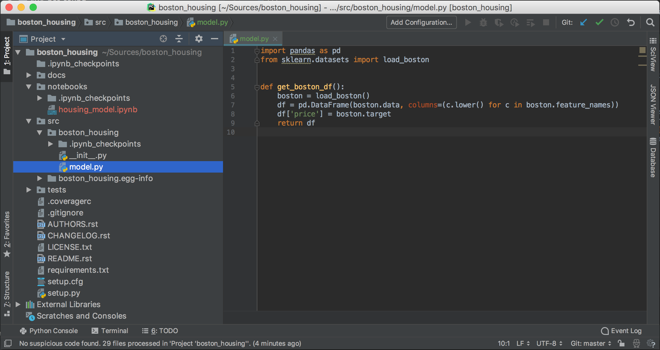
notebooks folder holds the notebooks for JupyterLab while the src/boston_housing folder contains the actual code (model.py) and defines an actual Python package.
If we use an IDE for development we will run into an obvious problem. How can we modify a function in our package and have these modifications reflected in our notebook without restarting the kernel every time? At this point I want to introduce you to your new best friend, the autoreload extension. Just add in the first cell of your notebook
%load_ext autoreload
%autoreload 2
and execute. This extension reloads modules before executing user code and thus allows you to use your IDE for development while executing it inside of JupyterLab.
4. Know your tool
JupyterLab is a powerful tool and knowing how to handle it brings you many advantages. Covering everything would exceed the scope of this blog post and thus I will mention here only practices that I apply commonly.
Use Shortcuts to speed up your work.
Accel means Cmd on Mac and Ctrl on Windows/Linux.
| Command | Shortcut |
|---|---|
| Enter Command Mode | Esc |
| Run Cell | Ctrl Enter |
| Run Cell & Select Next | Shift Enter |
| Add Cell Above/Below | A / B |
| Copy/Cut/Paste Cell | C / X / V |
| Look Around Up/Down | Alt ⇧ / ⇩ |
| Markdown Cell | M |
| Code Cell | Y |
| Delete Cell Output | M, Y (workaround) |
| Delete Cell | D D |
| Toggle Line Numbers | Shift L |
| Comment Line | Ctrl / |
| Command Palette | Accel Shift C |
| File Explorer | Accel Shift F |
| Toggle Bar | Accel B |
| Fullscreen Mode | Accel Shift D |
| Close Tab | Ctrl Q |
| Launcher | Accel Shift L |
Quickly access documentation
If you have ever used a notebook or IPython you surely know that executing a command prefixed with ? gets you the docstring (and with ?? the source code). Even easier than that is actually moving the cursor over the command and pressing Shift Tab. This will open a small drop-down menu displaying the help that closes automatically after the next key stroke.
Avoid unintended outputs
Using ; in Python is actually frowned upon but in Jupyterlab you can put it to good use. You surely have noticed outputs like <matplotlib.axes._subplots.AxesSubplot at 0x7fce2e03a208> when you use a library like Matplotlib for plotting. This is due to the fact that Jupyter renders in the output cell the return value of the function as well as the graphical output. You can easily suppress and only show the plot by appending ; to a command like plt.plot(...);.
Arrange cells and windows according to your needs
You can easily arrange two notebooks side by side or in many other ways by clicking and holding on a notebook’s tab then moving it around. The same applies to cells. Just click on the cell’s number, hold and move it up or down.
Access a cell’s result
Surely you have experienced this facepalm moment when your cell with long_running_transformation(df) is finally finished but you forgot to store the result in another variable. Don’t despair! You can just use result = _NUMBER, e.g. result = _42, where NUMBER is the execution number of your cell, e.g. In [42], to access and save your result. An alternative to _NUMBER is Out[NUMBER].
Use the multicursor support
Why should you be satisfied with only one cursor if you can have multiple? Just press Alt while holding down your left mouse button to select several rows. Then type as you would normally do to insert or delete.
Activate line numbers
Let’s assume you have to debug a cell with lots of code, I know you wouldn’t have cells with tons of code so let’s say your colleague caused that mess. To find the line corresponding to the error output more easily, you can just hit Shift L to show the line numbers for a moment.
Search all available actions
The Command Palette is surely one of the most powerful features of JupyterLab. Just hit the shortcut Accel Shift C and use the incremental search to find whatever action you are looking for. No more browsing menu drop downs for minutes!
5. Create your personal notebook template
After I have been using notebooks for a while I realized that in many cases the content of the first cell looks quite similar over many of the notebooks I created. Still, whenever I started something new I typed down the same imports and searched StackOverflow for some Pandas, Seaborn etc. settings. Consequently, a good advise is to have a template.ipynb notebook somewhere that includes imports of popular packages and often used settings. Instead of creating a new notebook with JupyterLab you then just right-click the template.ipynb notebook and click Duplicate.
The content of my template.ipynb is basically:
import sys
import logging

import numpy as np
import scipy as sp
import sklearn
import statsmodels.api as sm
from statsmodels.formula.api import ols

%load_ext autoreload
%autoreload 2

import matplotlib as mpl
import matplotlib.pyplot as plt
%matplotlib inline
%config InlineBackend.figure_format = 'retina'

import seaborn as sns
sns.set_context("poster")
sns.set(rc={'figure.figsize': (16, 9.)})
sns.set_style("whitegrid")

import pandas as pd
pd.set_option("display.max_rows", 120)
pd.set_option("display.max_columns", 120)

logging.basicConfig(level=logging.INFO, stream=sys.stdout)
6. Document your analysis
A really old programmer’s joke goes like “When I wrote this code, only God and I understood what it did. Now… only God knows.” The same goes for an analysis or creating a predictive model. Therefore your future self will be very thankful for documentation of your code and even some general information about goals and context. Notebooks allow you to use Markdown syntax to annotate your analysis and you should make plenty use of it. Even mathematical expressions can be embedded using the $...$ notation. More general information about the whole project can be put into README.rst which was also created by PyScaffold. This file will also be used as long description when the package is built and thus be displayed by an artefact store like PyPI or devpi. Also GitHub and GitLab will display README.rst and thus provide a good entry point into your project. If you are more into the Markdown syntax and thus rather want a README.md, you can install the pyscaffoldext-markdown extension for PyScaffold which adds a --markdown flag to PyScaffold’s putup command.
The actual source code in your package should be documented using docstrings which brings us to a famous joke of Andrew Tanenbaum “The nice thing about standards is that you have so many to choose from”. The three most common docstring standards for Python are the default Sphinx RestructuredText, Numpy and Google style which are all supported by PyCharm. Personally I like the Google style the most but tastes are different and more important is to be consistent after you have picked one. In case you have lots of documentation which would blow the scope of a single readme file, maybe you came up with a new ML algorithms and want to document the concept behind it, you should take a look at Sphinx. Our project setup already includes a docs folder with an index.rst as a starting point and new pages can be easily added. After you have installed Sphinx you can build your documentation as HTML pages:
conda install spinx
python setup.py docs
It’s also possible to create a nice PDF and even serve your documentation as a web page using ReadTheDocs.
7. State your dependencies for reproducibility
Python and its ecosystem evolve steady and quick, thus things that worked today might break tomorrow after a version of one of your dependencies changed. If you consider yourself a data scientist, you should always guarantee reproducibility of whatever you do since it’s the most fundamental pillar of any real science. Reproducibility means that given the same data and code your future you and of course others should be able to run your analysis or model receiving the same results. To achieve this technically we need to record all dependencies and their versions. Using conda we can do this with our boston_housing project as:
conda env export -n boston_housing -f environment.lock.yaml
This creates a file environment.lock.yaml that recursively states all dependencies and their version as well as the Python version that was used to allow anyone to deterministically reproduce this environment in the future. This is as easy as
conda env create -f environment.lock.yaml --force
Besides a concrete environment file that exhaustively lists all dependencies, it’s also common practice to define an environment.yaml where you state your abstract dependencies. These abstract dependencies comprise only libraries which are directly imported with no specific version. In our case this file looks like:
name: boston_housing
channels:
  - defaults
dependencies:
  - jupyterlab
  - pandas
  - scikit-learn
  - seaborn
This file keeps track of all libraries you are directly using. If you added a new library you can use this file to update your current environment with:
conda env update --file environment.yaml
Remember to regularly update and commit changes to these files in Git. Whenever you are satisfied with an iteration of your work also make use of Git tags in order to have reference points for later. These tags will also be used automatically as version numbers for your Python package which is another benefit of having used PyScaffold for your project setup.
Reproducible environments are only one aspect of reproducibility. Since many machine learning algorithms (most prominently Deep Learning) use random numbers it’s important to keep them deterministic by fixing the random seed. This sounds easier at it is since depending on the used framework, there are different ways to accomplish this. A good overview for many common frameworks is provided in the talk Reproducibility, and Selection Bias in Machine Learning.
8. Develop locally, execute remotely
Quite often when you want to do some heavy lifting, your laptop won’t be enough and thus you might use some powerful workstation by remote access. Running JupyterLab on the workstation and accessing it, maybe through some SSH tunnel, is no problem at all but how can we now work on the modules in our package? One way would be to run your IDE on the workstation but this comes potentially with many downsides depending on your connection. A flaky connection might lead to increased latencies when typing or reduced resolution. For this reason it’s best to do the actual coding locally in your IDE and sync every change automatically to the workstation where JupyterLab runs. The general setup for the workstation is analogue to the local setup. We git clone our repository and use the environment.lock.yaml to create the exact same environment which we run locally, followed by a python setup.py develop. If we now start JupyterLab within this environment we will be able to import our package.
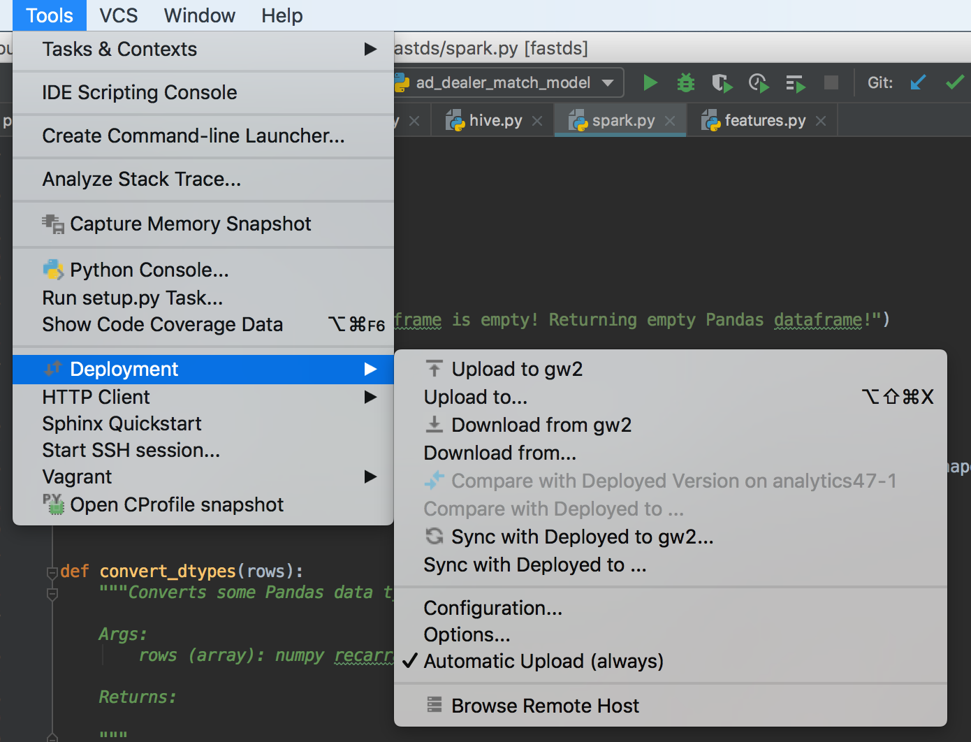
Now comes the interesting part: every change in one of our local modules needs to be reflected also on the remote workstation. You can use a classical command line tool like rsync for that or just rely on the features of your IDE. Over the last years I have grown quite fond of PyCharm’s Deployment feature as illustrated in Figure 2, which is unfortunately only available in the Professional version. It allows you to configure remote servers and if Automatic Upload is checked it syncs each file when saving. This convenient feature allows for blazing fast iterations. You make some changes to your model, maybe implement a new transformation function, hit Accel S to save, hit Accel Tab to switch to your browser with the JupyterLab tab and then rerun the modified model on the workstation.
From time to time, we also need to commit our changes using Git. Since we developed mostly on our local machine we only need to download the content of the notebooks folder from the remote workstation. For this we can again use rsync or the Download from … deployment feature of PyCharm Professional. Thus also all our git operations are executed locally avoiding merge conflicts between the local and remote repository. Git should not be used for syncing tasks anyway.
Another reason for running JupyterLab on a remote machine might be due to some firewall restrictions. Quite often in order to access sensitive data sources or a Spark cluster, you need to run JupyterLab on a gateway server. To invoke JupyterLab with Spark capabilities there are two ways. An ad hoc method is to just state on the command line that JupyterLab should use pyspark as kernel. For instance starting JupyterLab with Python 3.6 (needs to be consistent with your Spark distribution), 20 executors each having 5 cores might look like this:
PYSPARK_PYTHON=python3.6 PYSPARK_DRIVER_PYTHON="jupyter" PYSPARK_DRIVER_PYTHON_OPTS="notebook --no-browser --port=8899" /usr/bin/pyspark2 --master yarn --deploy-mode client --num-executors 20 --executor-memory 10g --executor-cores 5 --conf spark.dynamicAllocation.enabled=false
In order to be able to create notebooks with a specific PySpark kernel directly from JupyterLab, just create a file ~/.local/share/jupyter/kernels/pyspark/kernel.json holding:
{
 "display_name": "PySpark",
 "language": "python",
 "argv": [
  "/usr/local/anaconda-py3/bin/python",
  "-m",
  "ipykernel",
  "-f",
  "{connection_file}"
 ],
 "env": {
  "HADOOP_CONF_DIR": "/etc/hadoop/conf",
  "HADOOP_USER_NAME": "username",
  "HADOOP_CONF_LIB_NATIVE_DIR": "/var/lib/cloudera/parcels/CDH/lib/hadoop/lib/native",
  "YARN_CONF_DIR": "/etc/hadoop/conf",
  "SPARK_YARN_QUEUE": "dev",
  "PYTHONPATH": "/usr/local/anaconda-py3/bin/python:/usr/local/anaconda-py3/lib/python3.6/site-packages:/var/lib/cloudera/parcels/SPARK2/lib/spark2/python:/var/lib/cloudera/parcels/SPARK2/lib/spark2/python/lib/py4j-0.10.4-src.zip",
  "SPARK_HOME": "/var/lib/cloudera/parcels/SPARK2/lib/spark2/",
  "PYTHONSTARTUP": "/var/lib/cloudera/parcels/SPARK2/lib/spark2/python/pyspark/shell.py",
  "PYSPARK_SUBMIT_ARGS": "--queue dev --conf spark.dynamicAllocation.enabled=false --conf spark.scheduler.minRegisteredResourcesRatio=1 --conf spark.sql.autoBroadcastJoinThreshold=-1 --master yarn --num-executors 5 --driver-memory 2g --executor-memory 20g --executor-cores 3 pyspark-shell"
 }
}
Conclusion
We have seen that using an own Python package in conjunction with JupyterLab gives us means to program much cleaner and the ability to use a proper IDE. JupyterLab is a mighty and flexible tool and thus all the more it’s important to adhere to some best practices and processes to guarantee quality in your software and analysis. The boston_housing repository demonstrates a simple analysis of the Boston Housing Dataset in accordance with the outlined points above.
JupyterLab also offers many powerful extensions, e.g. jupyterlab-git, jupyterlab-toc, etc., for improved productivity that are worth checking out. If you have any additions or neat tricks for JupyterLab that were not covered, please let me know by using the comments below. Since general concepts are transferable but the specific workflow may be different, also read the blog post of Christopher Prohm about the same topic but using partly a different tooling.
Comments
comments powered by Disqus