Declarative Thinking and Programming

Motivation

Before we actually dive into this topic, imagine the following: You just moved to a new place and the time is ripe for a little house-warming dinner with your best friends Alice and Bob. Since Alice is really tech-savvy you just send her a digital invitation with date, time and of course your new address that she can add to her calendar with a single click. With good old Bob is a bit more difficult, he is having a real struggle with modern IT. That’s why you decide to send him an e-mail not only including the time and location but also a suggestion which train to take to your city, details about the trams, stops, the right street and so.

So let’s discuss the differences of how you interacted with Alice and Bob. We start by recalling what the actual task was. Your task was to organize a house-warming dinner with your friends. Therefore, your level of abstraction for that particular task should be on an organizing level. By sending the invitation message to Alice you declared that you want her to be at your place at a certain time not caring about how she is actually gonna accomplish this. With Bob it’s a completely different story. You not only declared your intentions but also provided lots of instructions on how to accomplish these. By doing so you left the level of organizing a dinner and went down to the task of planning a journey and this is not even the worst part. You also made a lot of error-prone assumptions that for instance Bob is gonna take the train to get to your city and not by some online ridesharing community which might have been a lot cheaper and faster.

Declarative Thinking

If we now transfer this example to programming we would describe the way of interaction with Alice as declarative and the interaction with Bob as imperative. So in a nutshell, declarative programming is writing code in a way that describes what you want to do and not how you want to do it. Sounds simple enough, right? But actually the difference between what and how is often not that clear. Is telling someone to take a particular train always telling someone how to do something and therefore imperative? No, actually not, it really depends on your actual task and the level of abstraction that comes with it.

Let’s say we want to do some linear algebra, in particular we want to sum up two n-dimensional vectors \(a\) and \(b\). Since we are in the domain of linear algebra using some computer algebra system (CAS), we would expect to be able to just declare what we want \(c = a + b\). Calculating \(c\) with the help of a loop would clearly be imperative in the given context. The downsides of using a loop for this are manifold. Firstly, we would define an implicit order of which elements to sum up first. This removes the possibility of our CAS software to choose a native SIMD CPU operation due to our over-specification of how to do it. Secondly, our code becomes much less readable and we are violating the single-level of abstraction as well as the separation of concerns principle which are both highly connected to declarative programming and thinking. If, on the other hand though, our task is to solve a given linear optimization problem, starting to implement a Simplex algorithm on our own with the help of vector operations in order to solve it can also be considered imperative.

Having realized the importance of the level of abstraction resp. the domain our task lives in, the obvious question is the following one: How do languages like SQL and Prolog or Datalog fit into our picture since they are always stated as being declarative? The first thing to note actually is that both languages are domain-specific languages (DSLs). Therefore they solely focus on solving problems in a single domain. For SQL that domain is querying a relational database. In order to fulfill this task the mathematical concept of a relational algebra was established borrowing from set theory. By using the relational algebra as toolbox to define queries we have an abstraction layer that is high-level, tailored to the task at hand but unsuitable for any other task outside that domain. The same observation holds for Prolog and Datalog which apply a set of mathematical concepts, most prominently the Horn clause, to solve problems in the field of logistic programming. At that point, it should also be noted that functional programming can also be considered to be declarative programming. Again, the abstraction layer is based on mathematical concepts with certain possible operations but also restrictions. For example a function is typically treated as any other value and can therefore be chained with other functions, passed as parameters or even returned from another function. Compared to an imperative language, the most well-known restriction is that functions are not allowed to have any side-effects.

Before we start to apply declarative concepts one word of caution about abstractions in general. In a perfect world an abstraction layer would completely hide the inner workings beneath it from the user. But even a DSL like SQL built on such a well-conceived theoretical foundation as the relational algebra is in practice a bit leaky. This can be experienced quite easily when looking at two different but logically equivalent queries differing in performance by orders of magnitude. The Law of Leaky Abstractions by Spolsky even states that “All non-trivial abstractions, to some degree, are leaky.” Beside this caveat, abstractions are still a powerful tool to handle complexity.

Declarative Programming

After having established some understanding of declarative programming and the general idea behind it, the focus is now to apply this to programming with Python. We start with some simple example. Let’s imagine we want the list of squared numbers from 1 to 10. The obvious approach would be:

result = []
for i in range(1, 11):
    result.append(i**2)

This surely is an imperative way of solving the problem. We have overspecified the problem in the sense that we dictate an order of how the solution should be calculated. We basically say in those few lines: “First square 1 and append the result to a list, then square 2 and so on”. By applying Python’s list comprehension feature we get much more closer to our actual question:

result = [i**2 for i in range(1, 11)]

Now we haven’t specified an ordering which would theoretically even allow the Python interpreter to calculate the result in parallel. Besides the list comprehension similar syntax exists for dictionaries and even sets.

Speaking about sets, the set type might even be the most underappreciated data type in Python’s standard library. Image you want to check if some sentences in a newly published paper exactly match sentences in your paper to prove plagiarism. Of course there a special tools for that but assume you have only Python. The naive approach would be to take a sentence from the first paper and compare it to all sentences of the other. Since this algorithm would be of complexity \(O(n^2)\) the performance would be quite bad if you want to check two extensive papers. So how would one apply declarative thinking here? The first and actual hardest part is to realise that we are dealing with a problem from set theory, i.e. we are not interested in the order of sentences nor the fact that there might be duplicates. Therefore we can apply set theory as abstraction layer and treat our paper as set \(A\) of sentences and the other as set \(B\). By doing so we are able to now express what we want in a single declaration \(A\cap B\) or equivalently in Python:

result = A & B

Again, we have not only gained readability compared to a version with two nested loops that I skipped here but execution will also be much faster since specialised algorithms based on hash tables are applied beneath the abstraction. In general, since Python provides so many built-in abstract datatypes, a good advise is to study them thoroughly in order to fully understand what they are capable of. For instance a dictionary seems to be something quite simple but realizing that a dictionary is actually a mathematical mapping allows us for instance to write an elegant dispatcher. Let’s assume first an imperative version:

def dispatch(arg, value):
    if arg == 'optionA':
        function_a(value)
    elif arg == 'optionB':
        function_b(value)
    elif arg == 'optionC':
        function_c(value)
    else:
        default(value)

What we actually want to say is that each argument maps to a function which is then called with a certain value like

dispatch = {'optionA': function_a,
            'optionB': function_b,
            'optionC': function_c}
dispatch.get(arg, default)(value)

Another often encounter that is deeply woven into Python is configuration via a Python module. Libraries like Sphinx, Python’s setuptools and many others use actual Python modules in order to configure certain settings. While this allows for utmost flexibility, their configuration files are often hard to read and error-prone. An declarative approach for configuration is the usage of a markup language like for instance YAML. Using YAML files to configure a Python program has several advantages. Firstly, any decent editor is able to parse it and therefore will warn you about syntax errors. Secondly, the format maps to Python’s dictionary data type and therefore many other libraries (e.g. data validation library like Voluptuous) which work on dictionaries can be easily applied. C and C++ have a long history of declarative build automation with the help of make and its declarative Makefiles. Also Rust’s build and packaging tool cargo is applying a declarative markup language, namely TOML. The take-away message is plain and simple. Prefer a markup language over a Python module for configuration in case you don’t need the extra flexibility of a whole programming language.

When it comes to parallel programming in Python declarative programming might also come in handy. Again, everything stands and falls with the actual use-case, but let’s assume that we have several tasks in the form of pure functions, i.e. functions without any side effects. Furthermore, some tasks depend on the result of others while others could be potentially executed in parallel. Imperatively we could use Python’s multiprocessing module to run certain tasks in parallel, synchronize when necessary and make sure we don’t get confused in the bookkeeping. Thinking about the problem at hand, a declarative programmer would realise that a directed acyclic graph (DAG) together with some mathematical concepts like topological ordering will form a suitable abstraction layer for a scheduling problem like that. This epiphany would lead him directly to a nice tool called Dask that allows to define and run a DAG in a declarative way. Also TensorFlow follows a similar approach to provide means for parallel, linear algebra that is mostly used for deep learning. At the same time newer versions also provide another abstraction layer that allows the declaration of neural network layers just like Keras. Here we can see that larger software packages even provide several abstraction layers built on eachother and let the user decide which abstraction is suitable for the task at hand. Another example for this is SQLAlchemy with its core and ORM layers.

At this point you surely got the hang of it. The essence of declarative programming is describing a problem within its domain applying high-level concepts thus focusing more on the what and less on the how. This allows us to increase the readability of our code, quite often reduce the number of programming errors and also increase the performance at least compared to a naive implementation. To conclude this post let’s take a look at a fancier example from the domain of logic. We want to apply declarative programming to solve one of the Logelei riddles of the renowned german newspaper Die Zeit.

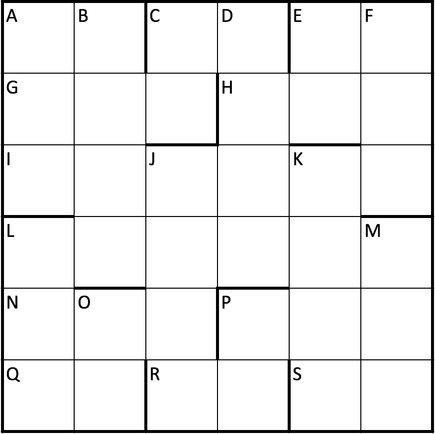
horizontal:
A: digit sum of horizontal C, C: prime number, E: palindrome, G: multiple of the backward number of horizontal A, H: all digits are equal, I: vertical F times vertical K, L: multiple of vertical M, N: multiple of horizontal Q, P: vertical B is a multiple, Q: square number, R: square number, S: prime number.

vertical:
All numbers are square numbers.

Solving such a problem with Python’s common tools and libraries is possible but also quite cumbersome. Since we know that this problem is a problem from the domain of formal logic, there is actually no reason to leave this abstraction layer. With that in mind, the riddle can just be seen as a set of rules and facts. For instance we know for a fact that a number consist of digits 0 to 9 with the first digit being from 1 to 9. An example for a rule would be that an integer \(n\) is a square number if and only if there exists an integer \(k\) so that \(k^2=n\). We will use the Python library PyDatalog to translate the riddle into a proper form so that, after having stated all facts and rules, we can just ask for the values of each field of the table and PyDatalog will do the inference based on the knowledge we have given. The syntax of PyDatalog might seem a bit strange at first but it is really concise and powerful. The rule for a square number is stated as:

squared(X) <= (math.sqrt(X).is_integer() == True)

It’s best to read the leftmost <= as if. So the line above states that a number \(X\) is squared if \(\sqrt{X}\in\mathbb{N}\). In an analogous manner, we can define a rule if one number is divisible by another with:

divisible(X, Y) <= (divmod(X, Y)[1] == 0)

Defining the rule for a prime number is a bit more tricky:

+prime(2)
+prime(3)
prime(X) <= (X > 3) & ~divisible(X, 2) & ~factor(X, 3)
factor(X, Y) <= divisible(X, Y)
factor(X, Y) <= (Y+2 < math.sqrt(X)) & factor(X, Y+2)

The first two lines add the facts that \(2\) and \(3\) are prime numbers to our knowledge. The third line says that any number \(X\) is a prime number if it is greater than \(3\), if it is not divisible by \(2\) and if it has not any other factor greater or equal than \(3\). To express the notion of any other factor greater or equal than 3, we have to apply recursion. From high school we know that in order to find out if an odd number is prime, we should check all odd numbers from \(3\) to \(\sqrt{X}\) if any of them is a factor of \(X\). This is exactly what the fifth line does. Here, an upper search boundary is defined and the recursion step itself. Since we start with the factor candidate \(3\) (as in line 3), the recursion iterates over all odd numbers up to \(\sqrt{X}\). Easy, right?

Let’s denote each field in our table with a coordinate where rows are A to F and columns 0 to 5 for easier reference. Since each field holds a digit but our rules and many constraints of the riddle are defined for numbers we have to map digits to the corresponding number. This can be done easily in PyDatalog with:

num[A, B] = 10*A + B
num[A, B, C] = 10*num[A, B] + C
num[A, B, C, D] = 10*num[A, B, C] + D
num[A, B, C, D, E] = 10*num[A, B, C, D] + E
num[A, B, C, D, E, F] = 10*num[A, B, C, D, E] + F

Now we are all set to translate the riddle one constraint after another to PyDatalog. Unfortunately, that’s where things will go crazy due to leaky abstraction. Of course in theory everything should work but behind the curtain what PyDatalog will do is generating and eliminating possible solution candidates and if it does this in the wrong order computation could take forever if not some out of memory error bites us first. Putting a bit of thought into the riddle first, you could try to reorder the given constraints in a way that the list of solutions fulfilling the constraints stays low at all time. We accomplish this by partitioning the table into four corner parts and define the constraints for each of them separately like shown in the picture below:

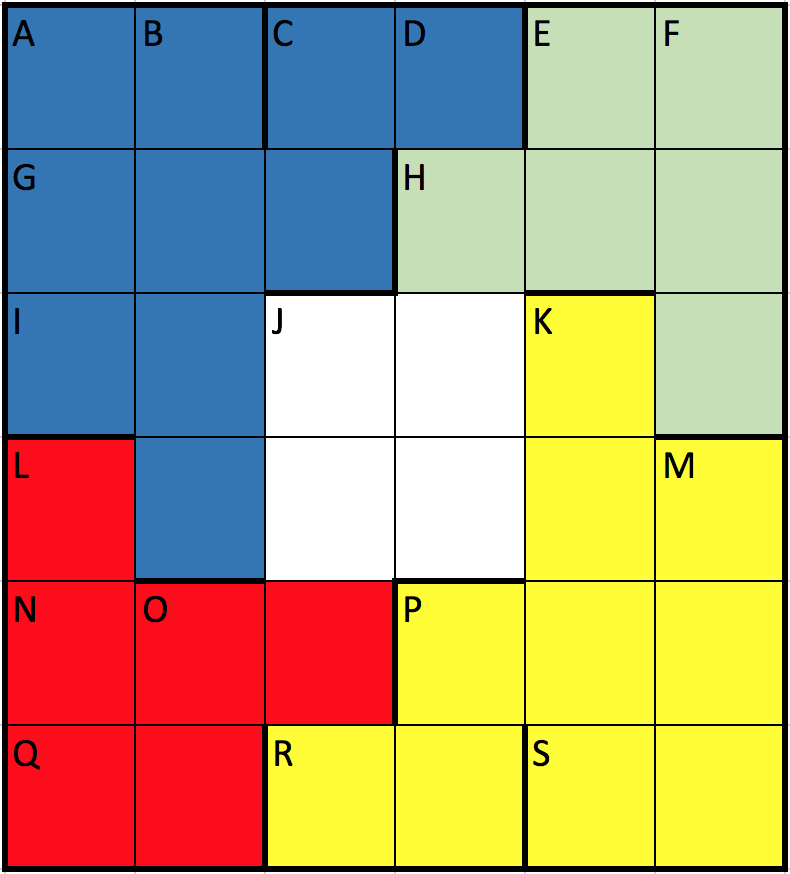
For the upper left, blue corner we can now define the set of all solutions with:

ul(A0, A1, A2, A3, B0, B1, B2, C0, C1, D1) <= (
    # C horizontal
    A2.in_(range(1, 10)) & A3.in_(range(1, 10)) & prime(num[A2, A3]) &
    # A horizontal
    A0.in_(range(1, 10)) & A1.in_(range(1, 10)) & (num[A0, A1] == A2 + A3) &
    # C vertical
    B2.in_(range(10)) & squared(num[A2, B2]) &
    # G horizontal
    B0.in_(range(1, 10)) & B1.in_(range(10)) & divisible(num[B0, B1, B2], num[A1, A0]) &
    # A vertical
    C0.in_(range(1, 10)) & squared(num[A0, B0, C0]) &
    # B vertical
    C1.in_(range(10)) & D1.in_(range(10)) & squared(num[A1, B1, C1, D1]))

The code is pretty much self-explanatory. For instance, the constraint C says that the fields A2 and A3 should form a prime number. Additionally, A2 and A3 are first digits of two different numbers in our table which means they can only be 1 to 9.

Having defined all four parts we can just combine them to arrive at the final solution as shown in the code below. We have seen that declarative programming can be really powerful in that it improves readability, maintenance and separation in programming. The notion behind declarative programming is that for a given task the level of abstraction should be applied allowing to describe the task in a canonical way.

import math
from pyDatalog import pyDatalog

pyDatalog.create_terms('math')
pyDatalog.create_terms('divmod')

@pyDatalog.program()
def _():
    squared(X) <= (math.sqrt(X).is_integer() == True)

    divisible(X, Y) <= (divmod(X, Y)[1] == 0)

    +prime(2)
    +prime(3)
    prime(X) <= (X > 3) & ~divisible(X, 2) & ~factor(X, 3)
    factor(X, Y) <= divisible(X, Y)
    factor(X, Y) <= (Y+2 < math.sqrt(X)) & factor(X, Y+2)

    # convert digits to number
    num[A, B] = 10*A + B
    num[A, B, C] = 10*num[A, B] + C
    num[A, B, C, D] = 10*num[A, B, C] + D
    num[A, B, C, D, E] = 10*num[A, B, C, D] + E
    num[A, B, C, D, E, F] = 10*num[A, B, C, D, E] + F

    # rows are denoted with A, B, C, D, E, F
    # columns are denoted with 0, 1, 2, 3, 4, 5

    # upper left corner
    ul(A0, A1, A2, A3, B0, B1, B2, C0, C1, D1) <= (
        # C horizontal
        A2.in_(range(1, 10)) & A3.in_(range(1, 10)) & prime(num[A2, A3]) &
        # A horizontal
        A0.in_(range(1, 10)) & A1.in_(range(1, 10)) & (num[A0, A1] == A2 + A3) &
        # C vertical
        B2.in_(range(10)) & squared(num[A2, B2]) &
        # G horizontal
        B0.in_(range(1, 10)) & B1.in_(range(10)) & divisible(num[B0, B1, B2], num[A1, A0]) &
        # A vertical
        C0.in_(range(1, 10)) & squared(num[A0, B0, C0]) &
        # B vertical
        C1.in_(range(10)) & D1.in_(range(10)) & squared(num[A1, B1, C1, D1]))

    # upper right corner
    ur(A4, A5, B3, B4, B5, C5) <= (
        # E horizontal
        A4.in_(range(1, 10)) & A5.in_(range(1, 10)) & (A4 == A5) &
        # H horizontal
        B3.in_(range(1, 10)) & B4.in_(range(10)) & B5.in_(range(10)) & (B3 == B4) & (B4 == B5) &
        # E vertical
        C5.in_(range(10)) & squared(num[A4, B5]) &
        # F vertical
        squared(num[A5, B5, C5]))

    # lower left corner
    ll(D0, E0, E1, E2, F0, F1) <= (
        # Q horizontal
        F0.in_(range(1, 10)) & F1.in_(range(10)) & squared(num[F0, F1]) &
        # O vertical
        E1.in_(range(1, 10)) & squared(num[E1, F1]) &
        # N horizontal
        E0.in_(range(1, 10)) & E2.in_(range(10)) & divisible(num[E0, E1, E2], num[F0, F1]) &
        # L vertical
        D0.in_(range(1, 10)) & squared(num[D0, E0, F0]))

    # lower right corner
    lr(A0, A1, A2, A3, B0, B1, B2, C0, C1, C4, D1, D4, D5, E3, E4, E5, F2, F3, F4, F5) <= (
        # fulfill upper left corner in order to have B vertical
        ul(A0, A1, A2, A3, B0, B1, B2, C0, C1, D1) &
        # S horizontal
        F4.in_(range(1, 10)) & F5.in_(range(10)) & prime(num[F4, F5]) &
        # M vertical
        D5.in_(range(1, 10)) & E5.in_(range(10)) & squared(num[D5, E5, F5]) &
        # P vertical
        E3.in_(range(1, 10)) & F3.in_(range(10)) & squared(num[E3, F3]) &
        # P horizontal
        E4.in_(range(10)) & divisible(num[A1, B1, C1, D1], num[E3, E4, E5]) &
        # R horizontal
        F2.in_(range(1, 10)) & squared(num[F2, F3]) &
        # K vertical
        C4.in_(range(1, 10)) & D4.in_(range(10)) & squared(num[C4, D4, E4, F4]))

    # complete riddle
    riddle(X) <= (
        # fulfill all corners and connect them
        ul(X[0][0], X[0][1], X[0][2], X[0][3], X[1][0], X[1][1], X[1][2], X[2][0], X[2][1], X[3][1]) &
        ur(X[0][4], X[0][5], X[1][3], X[1][4], X[1][5], X[2][5]) &
        lr(X[0][0], X[0][1], X[0][2], X[0][3], X[1][0], X[1][1], X[1][2], X[2][0], X[2][1], X[2][4],
           X[3][1], X[3][4], X[3][5], X[4][3], X[4][4], X[4][5], X[5][2], X[5][3], X[5][4], X[5][5]) &
        ll(X[3][0], X[4][0], X[4][1], X[4][2], X[5][0], X[5][1]) &
        X[2][2].in_(range(1, 10)) & X[2][3].in_(range(10)) &
        # I horizontal
        (I == num[X[2][0], X[2][1], X[2][2], X[2][3], X[2][4], X[2][5]]) &
        (F == num[X[0][5], X[1][5], X[2][5]]) &
        (K == num[X[2][4], X[3][4], X[4][4], X[5][4]]) &
        (I == F*K) &
        X[3][3].in_(range(1, 10)) &
        # D vertical
        squared(num[X[0][3], X[1][3], X[2][3], X[3][3]]) &
        X[3][2].in_(range(1, 10)) &
        # L horizontal
        (L == num[X[3][0], X[3][1], X[3][2], X[3][3], X[3][4], X[3][5]]) &
        (M == num[X[3][5], X[4][5], X[5][5]]) &
        divisible(L, M) &
        # J vertical
        squared(num[X[2][2], X[3][2], X[4][2], X[5][2]]))

    print(riddle([(A0, A1, A2, A3, A4, A5), (B0, B1, B2, B3, B4, B5), (C0, C1, C2, C3, C4, C5),
                  (D0, D1, D2, D3, D4, D5), (E0, E1, E2, E3, E4, E5), (F0, F1, F2, F3, F4, F5)]))

The last line above tells PyDatalog to just output all digits fulfilling the constraints of our riddle:

A0 | A1 | A2 | A3 | A4 | A5 | B0 | B1 | B2 | B3 | B4 | B5 | C0 | C1 | C2 | C3 | C4 | C5 | D0 | D1 | D2 | D3 | D4 | D5 | E0 | E1 | E2 | E3 | E4 | E5 | F0 | F1 | F2 | F3 | F4 | F5
---|----|----|----|----|----|----|----|----|----|----|----|----|----|----|----|----|----|----|----|----|----|----|----|----|----|----|----|----|----|----|----|----|----|----|---
1  | 1  | 4  | 7  | 2  | 2  | 4  | 2  | 9  | 5  | 5  | 5  | 4  | 9  | 5  | 6  | 1  | 6  | 6  | 6  | 1  | 9  | 9  | 1  | 7  | 6  | 8  | 4  | 3  | 2  | 6  | 4  | 4  | 9  | 6  | 1 

While this example might look like fun but actually not applicable for real work, this surely is not the case. Microsoft is applying Datalog for instance to check beliefs about dynamic networks and others use it for applications in program analysis, security and data integration. In general, systems to resolve constraints and dependencies are used in NixOS which got quite some traction over the last years since it allows package and configuration management in a declarative way. In a nutshell, it gives you ways to describe what your system should look like which is completely different compared to the usual way where you use for instance apt-get install to install packages in order to move your current state of your system to the desired one. As a user of a Linux system your actual concern is the set of programs or services that should be available to you, not so much what needs to be installed to move from one state to another.

There are many other examples of an imperative design versus a declarative design that solve the same problem, for instance the data pipline and workflow tools Airflow versus Luigi. So if your job is to solve a problem with the help of a program or framework, make sure to be absolute clear about what you want to accomplish. It often helps to put yourself into the role of a user to understand what needs to be declared in order to describe the problem. Only then start to think about a theoretical domain that might help you to achieve a declarative level of abstraction for your task. Declarative programming means finding the right abstraction level that describes your problem.

A talk covering this blog post was presented at the EuroPython 2017: